A Study on Comparison of Jacobi,
Gauss-Seidel and Sor Methods for the Solution in
System of Linear Equations
Dr.S.Karunanithi#1, N.Gajalakshmi#2, M.Malarvizhi#3 , M.Saileshwari*4#
Assistant Professor ,* Research Scholar Thiruvalluvar University,Vellore
PG & Research Department of Mathematics,Govt.Thirumagal Mills College,Gudiyattam,Vellore Dist,Tamilnadu,India-632602
Abstract —This paper presents three iterative methods for the solution of system of linear equations has been evaluated in this work. The result shows that the Successive Over-Relaxation method is more efficient than the other two iterative methods, number of iterations required to converge to an exact solution. This research will enable analyst to appreciate the use of iterative techniques for understanding the system of linear equations.
Keywords —The system of linear equations, Iterative methods, Initial approximation, Jacobi method, Gauss-Seidel method, Successive Over- Relaxation method.
1. INTRODUCTION AND PRELIMINARIES
Numerical analysis is the area of mathematics and computer science that creates, analyses, and implements algorithms for solving numerically the problems of continuous mathematics. Such problems originate generally from real-world applications of algebra, geometry and calculus, and they involve variables which vary continuously. These problems occur throughout the natural sciences, social science, engineering, medicine, and business.
The solution of system of linear equations can be accomplished by a numerical method which falls in one of two categories: direct or iterative methods. We have so far discussed some direct methods for the solution of system of linear equations and we have seen that these methods yield the solution after an amount of computation that is known advance.
We shall now describe the iterative or indirect methods, which start from an approximation to the true solution and, if convergent, derive the sequence of closer approximations-the cycle of computations being repeated till the required accuracy is obtained. This means that in a direct method the amount of computation is fixed, while in an iterative method the amount of computation depends on the accuracy required.
In general, one should prefer a direct method for the solution a linear system, but in the case of matrices with a large number of zero elements, it will be advantageous to use iterative methods which presents these elements.
2. PROBLEM FORMULATION
In this section, we consider the system of „n‟ linear equations in „n‟ unknowns is given by
………..……….. ………. (1) ………..……..
May be represented as the matrix equation, where
AX=B ……… (2) Where
A = X = And B =
In which the diagonal elements aij do not vanish. If this is not the case, then the equations should be rearranged,
……… ………....
In general, we have
…………. (3)
Now, if an initial guess x01, x02, x03……. x0n, for all the unknowns was available, we could substitute
these values into the right-hand side of the set of equations (3) and compute an updated guess for the unknowns, x11, x12, x13……. x1n. There are several ways to accomplish this, depending on how you use the most recently
computed guesses.
3. ITERATIVE METHODS
The approximate methods for solving system of linear equations makes it possible to obtain the values of the roots system with the specified accuracy. This process of constructing such a sequence is known as iteration. Three closely related method studied in this work are all iterative in nature. Unlike the direct methods, which attempts to calculate an exact solution in a finite number of operations, these methods starts with an initial approximation and generate successively improved approximations in an infinite sequence whose limit is the exact solution. In practical terms, this has more advantage, because the direct solution will be subject to rounding errors.
3.1 JACOBI METHOD
In numerical linear algebra, the Jacobi method is an algorithm for determining the solutions of a diagonally dominant system of linear equations. Each diagonal element is solved for, and an approximate value is plugged in. The process is then iterated until it converges. This algorithm is a stripped- down version of the Jacobi transformation method of matrix diagonalization.
In the Jacobi method, all of the values of the unknowns are updated before any of the new information is used in the calculations. That is, starting with the initial guess x01, x02, x03……. x0n, compute the next
approximation of the solution as
……… ………
Or, after k iterations of this process, we have
……… ………
This method is due to Jacobi and is called the method of simultaneous displacements.
3.2 GAUSS SEIDEL METHOD
In the first equation of equation (1), we substitute the first iterations x01, x02, x03……. x0n, into the
right-hand side and denote the results as x11 . In the second equation we substitute x11, x02, x03……. x0n, and denote the
result as x12 . In this manner, we complete the first stage of iteration and the entire processes is repeated till the
values of x1, x2, x3……. xn are obtained to the accuracy required. It is clear, therefore, that this method used an
improved component as shown as it is available and it is called the method of successive displacement (or) the Gauss-seidel method. If we implement this, our method would look like
……… ………
Or, after k iterations of this process, we have
……… ………
More generally
………… (5)
3.3 SUCCESSIVE OVER-RELAXATION (SOR)
In numerical linear algebra, the method of successive over-relaxation (SOR) is a variant of the Gauss-Seidel method for solving a system of linear equations, resulting in faster convergence. A similar method can be used for any slowly converging iterative process.
The successive over-relaxation (SOR), is devised by applying extrapolation to the Gauss-Seidel method. This extrapolation takes the form of a weighted average between the previous iterate and the computed iterate successively for each component.
= (1-ω) + ( ), i=1,2,3…..n ……… (6)
(where x denote a Gauss- Seidel iterate, and ω is the extrapolation factor). The idea is to choose a value for ω that will accelerate the rate of convergence of iterates to the solution.
If ω =1, the SOR method simplifies to the Gauss-Seidel method. Though technically the term under relaxation should be used when 0 < ω <1, for convenience the term over relaxation is now used for any value of ω Є (0,2).
4. CONVERGENCE OF ITERATIVE METHODS
The iterative methods converge, for any choice of the first approximation x0j (j=1,2,….), if every equation of
the system (1) satisfies the condition that the sum of the absolute values of the coefficients aij / aii almost equal
to, or in at least one equation less than unity.
Where the „<‟ sign should be valid in the case of „at least‟ one equation. It can be shown that the Gauss-Seidel method converges twice as fast as the Jacobi method.
5. ANALYSIS OF RESULTS
The efficiency of the three iterative methods was compared based on a 2x2, 3x3 and a 4x4 order of linear equations. They are as follows from the examples
EXAMPLE -1 Solve the system 5x + y = 10 2x +3y = 4
Using Jacobi, Gauss-Seidel and Successive Over-Relaxation methods.
SOLUTION
Given 5x + y = 10 2x +3y =4
The above equations can be written as the matrix form AX = B
= Let
A =
the given matrix A is diagonally dominant (i.e ),(ie 5≥1, 3≥2) hence, we apply the above said these iterative methods
To solve these equations by iterative methods, we are rewrite them as follows, x=
y= The results are given in the table -1(a)
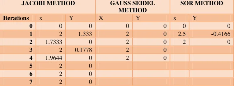
Table -1(a) Number of iterations of the iterative methods
JACOBI METHOD GAUSS SEIDEL
METHOD
SOR METHOD
Iterations x Y X Y x Y
0 0 0 0 0 0 0
1 2 1.333 2 0 2.5 -0.4166
2 1.7333 0 2 0 2 0
3 2 0.1778 2 0
4 1.9644 0 2 0
5 2 0
6 2 0
7 2 0
Table -1(b) Number of iterations for the SOR, GAUSS-SEIDEL AND JACOBI ITERATIVE METHODS
METHODS NUBMER OF TERATIONS
SOR METHOD 2
GAUSS SEIDEL METHOD 5
JACOBI METHOD 7
Number of iterations for the SOR, GAUSS-SEIDEL AND JACOBI ITERATIVE METHODS
EXAMPLE – 2 Solve the system
10x + 2y – z = 7
1x + 8y + 3z = -4
-2x – y + 10z = 9
Using Jacobi, Gauss-Seidel and Successive Over-Relaxation methods.
SOLUTION
Given 10x + 2y – z = 7
1x + 8y + 3z = -4
-2x – y + 10z = 9
The above equations can be written as the matrix form AX = B
=
Let
A =
the given matrix A is diagonally dominant (i.e ) , (ie10≥3, 8≥4, 10≥3) hence, we apply the above said these iterative methods
To solve these equations by iterative methods, we are rewrite them as follows, x=
y=
Table 2(a) – Number of iterations of the iterative methods
JACOBI METHOD GAUSS-SEIDEL METHOD SOR METHOD
Iterations X Y Z x Y Z X Y Z
0 0 0 0 0 0 0 0 0 0
1 0.7 -0.5 0.9 0.7 -0.5875 0.98125 0.77 -0.55 0.99
2 0.89 -0.925 0.99 0.9156 -0.9824 0.98488 0.9229 -1.0303 0.9807
3 0.984 -0.9825 0.9855 0.995 -0.9937 0.9996
4 0.9951 -0.9926 0.9986 0.9987 -0.9997 1.1997
5 0.9984 -0.9989 0.9998
6 0.99976 -0.9997 0.9998
7 0.9999 -0.9999 0.9999
8 0.9999 -0.9999 0.9999
9 0.9999 -0.9999 0.9999
10 0.9999 -0.9999 0.9999
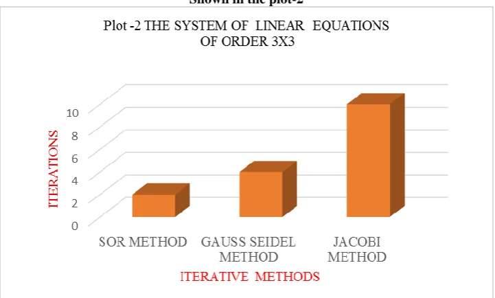
Table -2(b) Number of iterations for the SOR, GAUSS-SEIDEL AND JACOBI ITERATIVE METHODS
METHODS NUBMER OF ITERATIONS
SOR METHOD 2
GAUSS SEIDEL METHOD 4
JACOBI METHOD 10
Number of iterations for the SOR, GAUSS-SEIDEL AND JACOBI ITERATIVE METHODS
Shown in the plot-2
EXAMPLE – 3 Solve the system 10x1 – 2x2 – x3 – x4 = 3
-2x1 + 10x2 – x3 – x4 = 15
-x1 –x2 + 10x3 – 2x4 = 27
-x1 –x2 – 2x3 + 10x4 = -9
SOLUTION
Given 10x1 – 2x2 – x3 – x4 = 3
-2x1 + 10x2 – x3 – x4 = 15
-x1 –x2 + 10x3 – 2x4 = 27
-x1 –x2 – 2x3 + 10x4 = -9
The above equations can be written as the matrix form AX = B
10 -2 -1 -1 x1 3
-2 10 -1 -1 x2 15
-1 -1 10 -2 x3 = 27
-1 -1 -2 10 x4 -9
Let
10 -2 -1 -1
-2 10 -1 -1 A= -1 -1 10 -2
-1 -1 -2 10
the given matrix A is diagonally dominant (i.e ),(ie10≥4, 10≥4, 10≥4, 10≥4) hence, we apply the above said these iterative methods
To solve these equations by iterative methods, we are rewrite them as follows, = (3+2 x2+ x3 + x4)
= (15+2 x1+ x3 + x4)
= (27+x1+ x2 + 2x4)
= (-9+ x1+ x2 + 2x3)
The results are given in the table 3(a)
Table 3(a)- Number of iterations of iterative methods
JACOBI METHOD GAUSS - SEIDEL METHOD SOR METHOD
Iterations x1 x2 x3 x4 x1 x2 x3 x4 x1 x2 x3 x4
0 0 0 0 0 0 0 0 0 0 0 0 0 1 0.3 1.5 2.7 -0.9 0.3 1.56 2.886 -0.1368 0.375 1.96875 3.6679 0.0849 2 0.78 1.74 2.7 -0.18 0.8869 1.9523 2.9566 -0.0248 1.2425 2.1625 3.0 0.0 3 0.9 1.9608 2.916 -0.108 0.9836 1.9899 2.9924 -0.0042
4 0.9624 1.9608 2.9592 -0.036 0.9968 1.9982 2.9987 -0.0008 5 0.9845 1.9848 2.9851 -0.0158 0.9994 1.9997 2.9998 -0.0001 6 0.9939 1.9938 2.9938 -0.006 0.9999 1.9999 3.0 0.0 7 0.9975 1.9975 2.9976 -0.0025 1.0 2.0 3.0 0.0 8 0.9990 1.9990 2.9990 -.0010
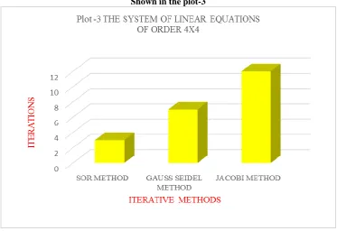
Table -3(b) Number of iterations for the SOR, GAUSS-SEIDEL AND JACOBI ITERATIVE METHODS
METHODS NUMBER OF ITERATIONS
SOR METHOD 3
GAUSS SEIDEL METHOD 7
JACOBI METHOD 12
Number of iterations for the SOR, GAUSS-SEIDEL AND JACOBI ITERATIVE METHODS
Shown in the plot-3
COMPARISION AND RESULTS
Number of iterations for the SOR, GAUSS-SEIDEL AND JACOBI ITERATIVE METHODS
Shown in the plot-4
CONCLUSION
The number of iterations differ, as that of the Successive-Over Relaxation method of order 4x4 has 3 iterations, while Gauss-Seidel has 7 iterations. This shows that Successive-Over Relaxation requires less iteration than the Gauss-Seidel method. Thus, the Successive-Over Relaxation could be considered more efficient of the three methods.
REFERENCES
1. Beale, I.M. (1988). „Introduction to Optimization‟ Published by John Wiley and Sons. Ltd.
2. Black, Noel; Moore, Shirley; and Weisstein, Eric W. Jacobi method. MathWorld.
3. Book Numerical analysis Vol. (3), pp- 226-258.
4. Demidovich B,maron I,The basics of numerical methods.Moscau:Nauka;1970.(in Russian)
5. Frienderg, S.H, Spence B.E. (1989). „Linear Algebra‟ 2nd Edition. Prentice Hall International Editions.
6. Jacobi method from www.math-linex.com
7. Kalambi, I.B. (1998). „Solutions of Simultaneous Equations by Iterative Methods‟. Postgraduate Diploma in Computer Science Project. Abubakar Tafawa Balewa University, Bauchi
8. Milaszewicz P. (1981), “Improving Jacobi and Gauss-Seidel Iterations can be applied to solve systems of linear equations, a natural questions how convergence rates are affected if the original”. SIAM Journal of Science Mathematics Computer Vol. (2), pp. 375-383.
9. Naeimi Dafchahi F. (2008), “A new Refinement of Jacobi Method for Solution of Linear System of equations”. Institute Journal of computer Mathematical Sciences, Vol. (3), pp. 819-827.
10. Niki H. (2004), “The survey of pre conditioners used for accelerating the rate of convergence in the Gauss-Seidel method.” Journal of Computer Applied Mathematics Vol. (113), pp. 164-165.
11. Ridgway Scott L. (2011), “Numerical solution of linear equation solve by Direct and Iterative methods.”
12. Rajasekaran,S. (1992). „Numerical methods in Science and Engineering. A practical approach. Wheelerand Co. Ltd Allahabad.
13. Turner, P.R. (1989). „Guide to Numerical Analysis‟ Macmillan Education Ltd. Hong Kong.
14. Turner, P.R. (1994). „Numerical Analysis‟. Macmillian Press Ltd. Houndsmills.