Computation of Various Queue Characteristics using Tri-Cum Biserial Queuing Model Connected with a Common Server

(1)

Computation of Various Queue Characteristics

using Tri-Cum Biserial Queuing Model

Connected with a Common Server

Sachin Kumar Agrawal1, B. K. Singh2

1

Research Scholar, Department of Mathematics, IFTM University, Moradabad, Uttar Pradesh, India

2

HOD, Department of Mathematics, IFTM University, Moradabad, Uttar Pradesh, India

Abstract: The present paper deals with the investigation of various characteristics of a developed queuing model in which three servers are connected in parallel in tri-cum biserial way with a common server. The arrival and service pattern are assumed to follow the Poisson law. Queue length, variance, average waiting time and probabilities have been estimated using statistical tools, generating function technique and law of calculus. Extensive parametric study has been presented to show the efficacy of the present solution methodology. Present study demonstrates that the queuing theory provides a good approach to analyze the complicated probabilistic and deterministic systems.

Keywords: Queuing model, Poisson law, Variance, Probabilities.

I. INTRODUCTION

Queuing theory has been widely used in the traditional service trade such as in supermarkets, restaurants, manufacturing processes, bus scheduling and hospital appointment bookings etc. One of the anticipated advantages from studying queuing systems is the assessment of the effectiveness of models in terms of utilization of the resources and waiting length. Consequently optimize the number of queues such that customers need not to wait longer when servers are too busy. Several literatures are available dealing with the realistic problems based on various queuing models. Jacksons [1] investigated the various characteristics of a queue system encompassing phase type service. Maggu [2] emphasized on phase type service queues with two servers in biseries to study the queue model. Singh et al [3] used parallel biserial queues to examine the transient behavior of a queuing network. Gupta et al [4] presented an extensive parametric study to explore the queuing model consist of biserial and parallel channels associated with a common server.

The state characteristics of a queue model having two subsystems with bi-serial channels connected with a common channel has been investigated by Kumar et al [5]. Gupta et al [6] presented a detailed investigation on the linkage of a flowshop scheduling model with a parallel biserial queue network. This work has been further explored by Seema et al [7] to optimize total flow time, waiting time and service time.

II. APPLICATION IN REAL TIME DOMAIN

Queuing theory can be implemented to a diversity of operational situations where it is not possible to precisely calculate the arrival rate (or time) of customers and service rate (or time) of service facilities. For example: In shopping mall, there are several sections such as electronic, garments, food etc. The customer entered in the mall can avail all the facilities available in the mall or can also enjoy some of them. It depends on the time available with the customer and the crowed in difference sections. Such problems can be dealt easily using present model.

III. MATHEMATICAL MODEL

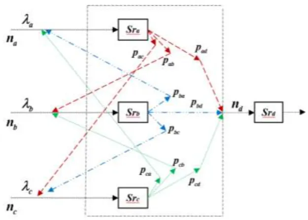
In the present work, a queue model consist of three servers (Sra, Srb and Src) are connected in parallel in tri-cum

biserial way which are further connected to a common server Srd. Let Qa, Qb ,Qc and Qd are the queues

associated with servers Sra, Srb, Src and Srd respectively. The number of customers (na) coming at mean arrival

rate (_a) after completion of service at server Sra, can avail the facility at server Srb or Src (either of two or both)

(2)

Fig 1: Linkage model of the queuing network

The governing differential difference equation in steady (transient) state of the model can be written as Eq. 1.

, , , 1, , , , 1, , , , 1,

1, 1, , 1, , 1, 1, , , 1

1, 1, , , 1, 1,

( )

a b c d a b c d a b c d a b c d

a b c d a b c d a b c d

a b c d a b c d

a b c a b c d n n n n a n n n n b n n n n c n n n n a a b n n n n a a c n n n n a a d n n n n b b a n n n n b b c n n n n b b

P P P P

p P p P p P

p P p P p

  

     

   

                  

     

      _, _1, _, ₁

, 1, 1, 1, , 1, , , 1, 1

, , , 1

a b c d

a b c d a b c d a b c d

a b c d

d n n n n c c b n n n n c c a n n n n c c d n n n n d n n n n

P

p P p P p P

P

 

     



     

 

(1)

Considering n_a  0; the Eq (1) can be given as

0 , , , 0 , 1, , 0 , , 1,

1, 1, , 1, , 1, 1, , , 1

0 , 1, 1, 0 , 1, , 1

0 , 1, 1, 0 , , 1,

( )

b c d b c d b c d

b c d b c d

b c d b c

a b c b c d n n n b n n n c n n n

a a b n n n a a c n n n a a d n n n b b c n n n b b d n n n

c c b n n n c c d n n n

P P P

p P p P p P

p P p P

 

  

   

  

              

     

   

    ₁

0 , , , 1

d

b c d

dP n n n





 

(2)

Considering n_b  0 ; the Eq (1) can be given as

, 0 , , 1, 0 , , , 0 , 1,

1, 0 , 1, 1, 0 , , 1

1, 1 , , , 1 , 1, , 1 , , 1

1, 0 , 1, , 0 , 1,

( )

a c d a c d a c d

a c d a c d

a c d a c d a c d

a c d a c

a b c a c d n n n a n n n c n n n

a a c n n n a a d n n n

b b a n n n b b c n n n b b d n n n c c a n n n c c d n n n

P P P

p P p P

p P p P p P

p P p P

 

   

  

  

              

   

     

    ₁

, 0 , , 1

d

a c d

dPn n n





 

(3)

, , 0 , 1, , 0 , , 1, 0 ,

1, 1, 0 , 1, , 0 , 1

1, 1, 0 , , 1, 0 , 1

, 1,1, 1, ,1, , ,1,

( )

a b d a b d a b d

a b d a b d

a b d a b d a b

a b c a b d n n n a n n n b n n n

a a b n n n a a d n n n b b a n n n b b d n n n

c c b n n n c c a n n n c c d n n n

P P P

p P p P

p P p P p P

                                  

      ₁

, , 0 , 1

d

a b d

dPn n n





 

(4)

Considering n_d 0 ; the Eq (1) can be given as

, , , 0 1, , , 0 , 1, , 0 3 , , 1, 0

1, 1, , 0 1, , 1, 0

1, 1, , 0 , 1, 1, 0

, 1, 1, 0 1, ,

( )

a b c a b c a b c a b c

a b c a b c

a b c a b c n n n a n n n b n n n n n n a a b n n n a a c n n n b b a n n n b b c n n n c c b n n n c c a n n n

P P P P

p P p P

                                      

    _{1, 0}

, , ,1

a b c

dPn n n



 

(5)

Considering n_a 0 & n_b 0; the Eq (1) can be given as

0 , 0 , , 0 , 0 , 1,

1, 0 , 1, 1, 0 , , 1

0 ,1, 1, 0 ,1, , 1

0 , 0 , 1, 1

0 , 0 , , 1

( )

c d c d

c d

a b c c d n n c n n

a a c n n a a d n n b b c n n b b d n n c c d n n

d n n

P P

p P p P

p P P                                (6)

Considering n_a 0 & n_c 0; the Eq (1) can be given as

0 , , 0 , 0 , 1, 0 ,

1, 1, 0 , 1, , 0 , 1

0 , 1, 0 , 1

0 , 1,1, 0 , ,1, 1

0 , , 0 , 1

( )

b d b d

b d

b d b d

b d

a b c b d n n b n n

a a b n n a a d n n b b d n n

c c b n n c c d n n d n n

P P

p P p P

p P

p P p P

P                                (7)

Considering n_a 0 & n_d 0; the Eq (1) can be given as

0 , , , 0 0 , 1, , 0 0 , , 1, 0

1, 1, , 0 1, , 1, 0

0 , 1, 1, 0

0 , , ,1

( )

b c b c b c

b c b c

b c

a b c b c n n b n n c n n

a a b n n a a c n n b b c n n

c c b n n d n n

P P P

p P p P

p P p P P                                (8)

Considering n_b 0 & n_c 0; the Eq (1) can be given as

, 0 , 0 , 1, 0 , 0 ,

1, 0 , 0 , 1

1, 1 , 0 , , 1 , 0 , 1

1, 0 ,1, , 0 ,1, 1

, 0 , 0 , 1

( )

a d a d

a d

a d a d

a d

a b c a d n n a n n a a d n n

b b a n n b b d n n c c a n n c c d n n d n n

P P

p P

p P p P

(4)

, 0 , , 0 1, 0 , , 0 , 0 , 1, 0

1, 0 , 1, 0

1, 1 , , 0 , 1 , 1, 0

1, 0 , 1, 0

, 0 , ,1

( )

a c a c a c

a c

a c a c

a c

a b c a c n n a n n c n n a a c n n

b b a n n b b c n n c c a n n

d n n

P P P

p P

p P p P

p P

P

 

 

 

 

            

 

   

 

(10)

Considering n_c 0 & n_d 0; the Eq (1) can be given as

, , 0 , 0 1, , 0 , 0 , 1, 0 , 0

1, 1, 0 , 0

, 1,1, 0 1, ,1, 0

, , 0 ,1

( )

a b a b a b

a b

a b a b

a b

a b c a b n n a n n b n n a a b n n

b b a n n

c c b n n c c a n n d n n

P P P

p P

p P p P

P

 

 

 

 

            

 

   

 

(11)

Considering n_a 0 ,n_b 0 & n_c 0; the Eq (1) can be given as

0 , 0 , 0 , 1, 0 , 0 , 1

0 ,1, 0 , 1

0 , 0 ,1, 1

0 , 0 , 0 , 1

( )

d d

d

a b c d n a a d n

b b d n

c c d n

d n

P p P

p P

P

   

        

 

(12)

Considering n_a 0 ,n_b 0 & n_d 0; the Eq (1) can be given as

0 , 0 , , 0 0 , 0 , 1, 0

1, 0 , 1, 0

0 ,1, 1, 0

0 , 0 , ,1

( )

c c

c

a b c c n c n

a a c n b b c n

d n

P P

p P

P 

 

        

 

(13)

Considering n_b 0 ,n_c 0 & n_d 0; the Eq (1) can be given as

, 0 , 0 , 0 1, 0 , 0 , 0

1, 1 , 0 , 0

1, 0 ,1, 0

, 0 , 0 ,1

( )

a a

a

a b c a n a n

b b a n c c a n d n

P P

p P

P 

 

        

 

(14)

Considering n_a 0 ,n_c 0 & n_d 0; the Eq (1) can be given as

0 , , 0 , 0 0 , 1, 0 , 0

1, 1, 0 , 0

0 , 1,1, 0

0 , , 0 ,1

( )

b b

b

a b c b n b n

a a b n c c b n

d n

P P

p P

P 

 

        

 

(15)

Considering n_a 0 ,n_b 0 ,n_c 0 & n_d 0; the Eq (1) can be given as

0 , 0 , 0 , 0 0 , 0 , 0 ,1

(5)

IV. SOLUTION METHODOLOGY

To solve the governing Equations, Generating function is assumed as

 1 2 3 4 1 2 3 4

0 0 0 0

, , , a b c d

a b c d

n n n n n n n n

f X X X X X X X X

   

   

     (17)

such that X1  X2  X3  X4 1

Also, taking partial generating function as

  , , ,

, , 1 1

0

n a n_a n_b n_c n_d b c d

a

n n n

n

f X P X





 _ (18)

  , ,  

, 1 2 1 2

0

, n_b n_c n_d . n b

c d

b

n n

n

f X X f X X





 _ (19)

 1 2 3 ,  1 2 3 0

, , n_c n_d , . n c

d

c

n

f X X X f X X X





 _ (20)

 1 2 3 4  1 2 3 4 0

, , , , , . n d

d

n

f X X X X f X X X X





 _ (21)

On solving equations from (1) to (16) with the help of (17), (18), (19), (20), (21), we get [2, 3]

 

   

     

2 3 4 1 3 4

1 1 1 2 2 2

1 2 4

1 2 4 1 2 3

3 3 3 4

1 2 3 4

2

1 2 3

1

1 , , 1 , ,

1

1 , , 1 , ,

, , ,

1 1 1 1

a b a c a d b a b c b d

a b

c a c b c d

c d

a b a c

a b c a

p X p X p X p X p X p X

f X X X f X X X

X X X X X X

p X p X p X

f X X X f X X X

X X X X

f X X X X

p X p

X X X

X                         _    _  _  _                 

    3 4

1 1

1 3 4 1 2 4

2 2 2 3 3 3 4

1

1 1 1

a d

b a b c b d c a c b c d

b c d

X p X

X X

X X X X X X X

              _    _ _    _ _  _         

Assuming f X2,X3,X4 fa, f X1,X3,X4 fb, f X1,X2,X4 fc, f X1,X2,X3 fd

 

     

2 3 4 1 3 4

1 1 1 2 2 2

1 2 4

3 3 3 4

1 2 3 4

2 3 4

1 2 3

1 1 1

1

1 1

1

1 1

, , ,

1 1 1 1

1

a b a c a d b a b c b d

a a b b

c a c b c d

c c d d

a b a c a d

a b c a

b a b

f f

X X X X X X

p X p X p X

f f

X X X X

f X X X X

p X p X p X

X X X

p X                         _    _  _  _              _    _            

 3 4 1 2 4

2 2 2 3 3 3 4

1

1 1

b c b d c a c b c d

c d

p X p X p X p X p X

X X X X X X X

                           

Since f(1, 1, 1, 1)  1, the total probability. Considering X1 1 as X2 1, X3 1, X4 1,

1 2 3 4

( , , , )

f X X X X is of (0/0) indeterminate form. Therefore, using L- Hospital rule, we get

(6)

Where, p_{a b}  p_{a c}  p_{a d} 1

afa  bpb afb cpc afc   a  a  bpb a cpc a

       (22)

Again differentiating numerator and denominator separately w.r.t. X2 by taking X2 1

as X1 1, X31, X4 1 , we get

     

1 a a b a b b a b c b d b c c b c

b a a b b b a b c b d c c b

p f p p p f p f

p p p p p

     



       

  

   

where p_{b a}  p_{b c} p_{b d} 1

apa bfa bfb cpc bfc b apa b b cpc b

        (23)

as X1 1, X2 1, X4 1 , we get

     

1 a a c a b b c b c c a c b c d c

c a a c b b c c c a c b c d

p f p f p p p f

p p p p p

     



       

  

   

where p_{c a}  p_{c b}  p_{c d} 1

apa c fa bpb cfb cfc c apa c bpb c c

        (24)

as X1 1, X2 1, X3 1 , we get

     

1 a a d a b b d b c c d c d d

a a d b b d c c d d

p f p f p f f

p p p

     



     

   

apa d fa bpb d fb cpc d fc d fd apa d bpb d cpc d d

         (25)

On solving (22) , (23), (24) and (25), we get:

                   1 1 1 1 1

a b c c b b b a b c c a c c a b c c b c b b a b c c a a

a a c c a b c c b a b a c c b b a b c c a

p p p p p p p p p p p p

f

p p p p p p p p p p

                                      1 1 1 1 1

a a b c a a c a c c b c a a b b c a a c c c b c a a b b

b b a a b c a a c b c b a a c c b c a a b

f

p p p p p p p p p p

                                     1 1 1 1 1

a a c a b b c b b c a b b a b a a c a b b c c a b b a c

c c b b c a b b a c a c b b a a c a b b c

f

p p p p p p p p p p

                                                     1 1 1 1 1 1 1 1 1

a b c c b b b a b c c a c c a b c c b c b b a b c c a a d

d a

d a a c c a b c c b a b a c c b b a b c c a

a a b c a a c a c c b c a a b b c a a c c c b c a a b b d

b

d b b a a b c a a c b c b a a c c

p f

p p p p p p p p p p

p

p p p p p p p p

                                                                    1 1 1 1

b c a a b

a a c a b b c b b c a b b a b a a c a b b c c a b b a c d

c

d c c b b c a b b a c a c b b a a c a b b c

p p

p

p p p p p p p p p p

                                   

The solution (Joint Probability) is written as

       

, , , 1 1 1 1

a b c d

n n n n

n n n n a b c d a b c d

(7)

       

, , , 1 1 1 1

a b c d a b c d

n n n n

n n n n a b c d a b c d

P             

where   _a 1 f_a,   _b 1 f_b,   _c 1 f_c, _d  1 f_d

        

       

 

1 1

a b c c b b b a b c c a c c a b c c b c b b a b c c a a

a a c c a b c c b a b a c c b b a b c c a

p p p p p p p p p p

      



    

  





   

     

       

 

1 1

a a b c a a c a c c b c a a b b c a a c c c b c a a b b

b b a a b c a a c b c b a a c c b c a a b

p p p p p p p p p p

      



    

  





        

       

 

1 1

a a c a b b c b b c a b b a b a a c a b b c c a b b a c

c c b b c a b b a c a c b b a a c a b b c

p p p p p p p p p p

      



    

  





        

       

 

   

     

       

 

1 1

a b c c b b b a b c c a c c a b c c b c b b a b c c a a d

d

d a c c a b c c b a b a c c b b a b c c a

a a b c a a c a c c b c a a b b c a a c c c b c a a b b d

d b a a b c a a c b c b a a c c b c a a b

p

p p p p p p p p p p

p

p p p p p p p p p p

        

  

    

 

 

       



    



  

 

  



        

       

 

1 1

a a c a b b c b b c a b b a b a a c a b b c c a b b a c d

d c b b c a b b a c a c b b a a c a b b c

p

p p p p p p p p p p



 

 _

        

  

    

 

 

  



The solution of this model exist if _a, _b, _c, _d 1 (26)

V. SYSTEM CHARECTERSTICS

(1) Mean queue length (average number of customers)

LQ  La Lb Lc Ld

1 1 1 1

a b c d

Q

a b c d

L        

       

Where , , ,

1 1 1 1

a b c d

L   L   L   L  

       

(2) Fluctuation (Variance) in queue length

Va r VaVb Vc Vd

 2  2  2  2

1 1 1 1

a b c d

a r

a b c d

V        

       

Where

 2 ,  2,  2,  2

1 1 1 1

a b c d

V   V   V   V  

       

(3) Average waiting time for customer

_{w t} Q , _{s u m} _a _b _c

s u m

L

E  w h e r e       

(8)

VI. PARAMETRIC STUDY

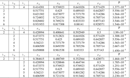
After developing the governing equations using mathematical model as discussed in section 3 and 4, following input parameters given in Table 1, have been used in the calculation of the results. In Table 2, various utilization of servers and joint probabilities have been shown for various values of mean arrival rate (_a

,band c). It is evident from the computed results that the values utilization of servers is less than 1 which

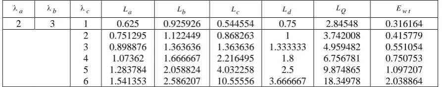
also satisfies Eq. (26). In Table 3 and Table 4, the average waiting time, queue lengths and variances have been calculated keeping different mean arrival rate (a ,band c) same as considered in Table 2.

Table 1: Various input parameters considered in computation of results

a

 _b _c _d p_{a b} p_{a c} p_{a d} p_{b a} p_{b c} p_{b d} p_{c a} p_{c b} p_{c d} n_a n_b n_c n_d

13 12 12 14 0.3 0.3 0.4 0.3 0.3 0.4 0.3 0.3 0.4 2 3 4 9

Table 2: Joint Probability and utilization of servers for various mean arrival rates

a

 _b _c _a _b _c _d P

1 3 4 0.414201 0.576923 0.641026 0.571429 1.377×10- 6

2 0.517751 0.625 0.689103 0.642857 5.556×10- 6

3 0.621302 0.673077 0.737179 0.714286 1.564×10- 5

4 0.724852 0.721154 0.785256 0.785714 3.018×10- 5

5 0.828402 0.769231 0.833333 0.857143 3.546×10- 5

6 0.931953 0.817308 0.88141 0.928571 1.546×10- 5

a

 _b _c _a _b _c _d P

2 1 4 0.428994 0.400641 0.592949 0.5 1.99×10- 7

2 0.473373 0.512821 0.641026 0.571429 1.308×10- 6

3 0.517751 0.625 0.689103 0.642857 5.556×10- 6

4 0.56213 0.737179 0.737179 0.714286 1.563×10- 5

5 0.606509 0.849359 0.785256 0.785714 2.667×10- 5

6 0.650888 0.961538 0.83333 0.57143 _1.450×10- 5

a

 _b _c _a _b _c _d P

2 3 1 0.384615 0.480769 0.352564 0.428571 1.464×10- 8

2 0.428994 0.528846 0.464744 0.5 1.785×10- 7

3 0.473373 0.576923 0.576923 0.571429 1.251×10- 6

4 0.517751 0.625 0.689103 0.642857 5.556×10- 6

5 0.56213 0.673077 0.801282 0.714286 1.562×10- 5

6 0.606509 0.721154 0.913462 0.785714 2.230×10- 5

Table 3: Average waiting time and queue lengths for various mean arrival rates

a

 _b _c L_a L_b L_c L_d LQ Ew t

1 3 4 0.707071 1.363636 1.785714 1.333333 5.189755 0.576639

2 1.07362 1.666667 2.216495 1.8 6.756781 0.750753

3 1.640625 2.058824 2.804878 2.5 9.004327 1.000481

4 2.634409 2.586207 3.656716 3.666667 12.544 1.393778

5 4.827586 3.333333 5 6 19.16092 2.128991

6 13.69565 4.473684 7.432432 13 38.60177 4.289086

a

2 1 4 0.751295 0.668449 1.456693 1 3.876437 0.430715

2 0.898876 1.052632 1.785714 1.333333 5.070556 0.563395

3 1.07362 1.666667 2.216495 1.8 6.756781 0.750753

4 1.283784 2.804878 2.804878 2.5 9.39354 1.043727

5 1.541353 5.638298 3.656716 3.666667 14.50303 1.611448

(9)

a

2 3 1 0.625 0.925926 0.544554 0.75 2.84548 0.316164

2 0.751295 1.122449 0.868263 1 3.742008 0.415779

3 0.898876 1.363636 1.363636 1.333333 4.959482 0.551054

4 1.07362 1.666667 2.216495 1.8 6.756781 0.750753

5 1.283784 2.058824 4.032258 2.5 9.874865 1.097207

6 1.541353 2.586207 10.55556 3.666667 18.34978 2.038864

Table 4: Variances for various mean arrival rates

a

 _b _c V_a V_b V_c V_d V_{a r}

1 3 4 1.20702 3.22314 4.97449 3.111111 12.51576

2 2.226279 4.444444 7.129344 5.04 18.84007

3 4.332275 6.297578 10.67222 8.75 30.05207

4 9.574517 9.274673 17.02829 17.11111 52.98859

5 28.13317 14.44444 30 42 114.5776

6 201.2665 24.48753 62.67348 182 470.4276

a

 _b _c V_a V_b V_c V_d V_{a r}

2 1 4 1.31574 1.115274 3.578647 2 8.009661

2 1.706855 2.160665 4.97449 3.111111 11.95312

3 2.226279 4.444444 7.129344 5.04 18.84007

4 2.931885 10.67222 10.67222 8.75 33.02632

5 3.917124 37.4287 17.02829 17.11111 75.48523

6 5.350419 650 30 42 727.34

a

 _b _c V_a V_b V_c V_d V_{a r}

2 3 1 1.015625 1.783265 0.841094 1.3125 4.952484

2 1.31574 2.382341 1.622145 2 7.320226

3 1.706855 3.22314 3.22314 3.111111 11.26425

4 2.226279 4.444444 7.129344 5.04 18.84007

5 2.931885 6.297578 20.29136 8.75 38.27083

6 3.917124 9.274673 121.9753 17.11111 152.2782

VII. CONCLUSION

In the present article a queuing model has been proposed and implemented to find the various characteristics of the queue network. Queue length, variance, Joint probability and average waiting time for customers have been computed using proposed mathematical model. The present model can be implemented in various stochastic and deterministic real time situations to have the accurate prediction of the systems.

REFERENCES

[1] Jackson, R.R.P. 1954. Queuing systems with phase-type service. Operational Research Quarterly, 5, 109-120.

[2] Maggu, P.L. 1970. Phase type service queues with two servers in biseries. Journal of Operational Research Society of Japan, 13(1), 1-6.

[3] Singh, T. P., Vinod, K., Rajinder, K., (2005). On transient behaviour of a queuing network with parallel biserial queues, JMASS, 1(2), 68-75.

[4] Gupta D., Singh, T.P., Rajinder, K., (2007). Analysis of a network queue model comprised of biserial and parallel channel linked with a common server.

Ultra Science, 19(2) M, 407-418.

[5] Kumar, V., Singh, T. P. , and Kumar, R. 2006. Steady state behaviour of a queue model comprised of two subsystems with biserial channels linked with a

common channel. Ref Des Era JSM, 1(2), 135-152.

[6] Gupta, D., Sharma, S. and Sharma, S. 2012. On linkage of a flowshop scheduling model including job block criteria with a parallel biserial queue network,

Computer Engineering and Intelligent System, 3(2), 17-28

(10)

Appendix

Symbol Notations

Servers S r_a,S rb,S rc,S rd

No. of Customers n_a,n_b,n_c,n_d

Mean arrival rates _a,_b,_c

Mean Service Rates _a, b, c,d

Probabilities p_{a b},p_{a c},p_{a d}

b a

p ,p_{b c} ,p_{b d} c a

p ,p_{c b} ,p_{c d}

Traffic intensity or utilization

of servers a

 ,b,c,d

Queue lengths L_a,Lb,Lc,Ld,LQ

Variances V_a,V_b,V_c,V_d ,V_{a r}

Average waiting time for

customers w t