Self-Paced Active Learning: Query the Right Thing at the Right Time

(1)

The Thirty-Third AAAI Conference on Artificial Intelligence (AAAI-19)

Self-Paced Active Learning: Query the Right Thing at the Right Time

Ying-Peng Tang, Sheng-Jun Huang

∗

College of Computer Science and Technology, Nanjing University of Aeronautics and Astronautics Collaborative Innovation Center of Novel Software Technology and Industrialization

Nanjing 211106, China {tangyp, huangsj}@nuaa.edu.cn

Abstract

Active learning queries labels from the oracle for the most valuable instances to reduce the labeling cost. In many ac-tive learning studies, informaac-tive and representaac-tive instances are preferred because they are expected to have higher poten-tial value for improving the model. Recently, the results in self-paced learning show that training the model with easy examples first and then gradually with harder examples can improve the performance. While informative and representa-tive instances could be easy or hard, querying valuable but hard examples at early stage may lead to waste of labeling cost. In this paper, we propose a self-paced active learning approach to simultaneously consider the potential value and easiness of an instance, and try to train the model with least cost by querying the right thing at the right time. Experimental results show that the proposed approach is superior to state-of-the-art batch mode active learning methods.

Introduction

In many real world applications, the amount of unlabeled data is far larger than that of labeled data; and label acquisition is expensive and difficult. It is thus rather important to train an effective model with fewer labeled examples. Active learning is one of the main approaches to deal with this challenge. It expects to reduce the labeling cost by selecting the most valuable instances to query their labels from the oracle (Set-tles 2009). During the past decades, many criteria have been proposed for active selection of instances. Among which, informativeness and representativeness are most frequently used, and their integration has been validated to be effective for selecting the most valuable instances (Wang and Ye 2013; Huang and Zhou 2013; Huang, Jin, and Zhou 2014).

All these criteria try to estimate the potential value of an instance on improving the model performance. However, they neglect the fact that the potential ability of a valuable instance may not be fully exploited at a specific stage of the model training. This phenomenon has been well validated in self-paced learning (SPL) (Kumar, Packer, and Koller 2010).

∗

This work was supported by National Key R&D Pro-gram of China (2018YFB1004300), NSFC (61503182, 61876081, 61732006).

Self-paced learning is inspired by the “easy to hard” pro-cess of human learning. It learns the easier instances first, and then gradually adds more complex instances for model into training. A typical SPL model tries to minimize a weighted sum of losses for all instances, where the weight reflects the easiness of an instance to the model. By optimizing the weights and the model alternately, instances are gradually involved from easy to hard. It has been well validated by many studies that this learning paradigm can lead to better generalization performances (Khan, Mutlu, and Zhu 2011; Tang, Yang, and Gao 2012; Basu and Christensen 2013; Zhang et al. 2016).

Based on these observations, it can be implied that at a specific training stage, over-complex examples may be less useful than easy ones for improving the model. On the other hand, while existing active learning methods focus on se-lecting informative and representative instances, they fail to query the right thing at the right time. Although the selected instances have high potential value for model improving, they may not be fully exploited at the current stage, and thus lead to waste of labeling cost. As a result, in addition to criteria estimating the potential value of improving the model, easi-ness of an instance to the current model should be considered in active selection.

In this paper, we propose a novel approach called SPAL (Self-Paced Active Learning) to simultaneously consider po-tential value and easiness of instances. On one hand, the selected instances should be informative and representative; on the other hand, they should not be over-complex for the current model, and thus can be fully utilized. Specifically, we maintain two weights for each unlabeled instance, one estimates the potential value on improving the model, and the other estimates how easily the model can fully exploit the potential value. Then by alternately optimizing the two weights, valuable and easy instances are selected. Further, when the model becomes stronger after more labels queried, harder instances can be gradually involved by increasing a pace parameter.

Experiments are performed on 9 datasets to validate the proposed approach. Results comparing with state-of-the-art methods show that considering the easiness of instances can boost the performance of active learning.

(2)

method is proposed next, followed by the experimental study. And at last we conclude this work.

Related Work

There are many selection criteria proposed for active learn-ing over the past few decades. Miscellaneous criteria eval-uate how useful an instance is for improving the model from different aspects. Most of them estimate the inmativeness or representativeness of the instance. The for-mer has been implemented by error reduction (Tang et al. 2012), query by committee (Seung, Opper, and Sompolin-sky 1992), uncertainty (Yan and Huang 2018), etc. While the latter has been implemented by clustering (Dasgupta and Hsu 2008) or density estimation (Zhu et al. 2010). Recently, it has been validated that simultaneously considering both the informativeness and representativeness is usually supe-rior to using a single criterion alone (Wang and Ye 2013; Huang and Zhou 2013; Huang, Jin, and Zhou 2014). Wang and ye (2013) optimize a well-designed objective function, which consists of a term estimating the uncertainty and a term estimating the distribution difference between labeled set and the whole data set. Huang et al. (2014) consider the min-max view of active learning (Hoi et al. 2008), and exploit both informativeness and representativeness with the help of unlabeled data in the semi-supervised learning setting. While all these methods try to estimate the potential value of an instance for improving the model, they neglect whether the selected example can be fully utilized by the current model. Learning concepts from easy to hard was first proposed in Curriculum learning (Bengio et al. 2009), in which the ‘cur-riculum’ is defined intuitively by human. Self-paced learning reformulates this learning process as an optimization prob-lem in order to make it more impprob-lementable. This algorithm alternately optimizes model and sample weights with a grad-ually increasing pace parameter, and sequentially involves instances from easy to hard. In the past few years, SPL has yielded brilliant results in many applications, such as vi-sual category discovery (Lee and Grauman 2011), long-term tracking (Supancic and Ramanan 2013), multi-view cluster-ing (Xu, Tao, and Xu 2015), multi-instance learncluster-ing (Zhang, Meng, and Han 2017). There are also a few works trying to integrate this paradigm into other algorithms for better per-formances. For example, Ma et al. (2017) propose self-paced co-training which aggregates SPL and co-training to improve the robustness. In (Wang et al. 2017), authors incorporate SPL with boosting method to deal with the noise sensitive problem.

There is one work trying to combine self-paced learning and active learning for face identification (Lin et al. 2018). This method on one hand employs self-paced learning to select instances with high confidence and assign them with pseudo labels predicted by the model; and on the other hand employs active learning to select most uncertain instances, and query their ground-truth labels from the oracle. However, these two strategies are employed independently, and thus still have the risk that the actively selected instances may not be fully utilized by the current model. Furthermore, the performance of this method heavily depends on the quality

of predicted labels, which could be unstable when the model is trained with very limited labeled data.

The Proposed Method

In this section, we first discuss the objective function of the proposed method and explain each term in the formula. Then, the optimization strategy is introduced next. And at last we present the steps of the algorithm.

We denote byDthe dataset withninstances, which in-cludes a small labeled set L = {(xi, yi)}ni=1l withnl

in-stances, and a large unlabeled setU ={xj}nj=l+nnl+1u withnu

instances, wherenlnuandn=nl+nu. At each iteration

of active learning, a small batch of instancesQ={xq}bq=1

with sizebwill be selected fromU to query their labels from the oracle.

The objective function

It has been disclosed by self-paced learning that learning from easy to hard can boost the performance. This implies that at a specific training stage, over-complex instances may be less useful for improving the model, and querying their labels can cause waste of labeling cost. While the informative and representative instances could be easy or hard for the current model, over-complex instances may not be fully utilized even they have high potential value. It is thus important to query the right thing at the right time. On one hand, the selected instances should have high potential value for improving the model; and on the other hand, the potential value can be fully exploited by the current model.

To achieve this goal, we introduce a variablewj∈[0,1]

for each unlabeled instancexjto estimate the potential value.

Specifically, more informative and representative instance should receive a higher value of wj. In addition, another

variablevj ∈[0,1]is introduced to estimate the easiness of

instancexjfor the current model. By employing a regularizer

imposed on this weight, easier sample will receive a largervj.

Then the following objective function is proposed to optimize the two variables along with the model:

min

f,w,v`(f,w,v) +λg(v) +µh(L∪Q, U\Q) +γΩ(f),

(1) wherefis the learning model. The first term calculates the expected loss after the query,g(·)is a self-paced regularizer to filter out over-complex instances,h(L∪Q, U\Q)is a func-tion to estimate the distribufunc-tion difference between labeled and unlabeled data, andΩ(f)is for controlling the model complexity. In summary,`(·),h(·)andg(·)are responsible for informativeness, representativeness and easiness, respec-tively.

Next, we specify the implementations of`(·),h(·)andg(·) in detail. For simplicity, we employ the least squared loss to estimate the expected losses of instances. And we will get the following form of`(·):

`(f,w,v) =

nl

X

i=1

(yi−f(xi))2+ nu

X

j=1

vjwj( ˆyj−f(xj))2.

(3)

One challenge here is the ground-truth labels of the se-lected data are unknown before querying. Inspired by (Wang and Ye 2013), we consider the upper bound of the risk by takingyˆj =−sign(f(xj))as the pseudo label ofxj ∈U.

Then we have the following expected loss with self-paced weights:

`(f,w,v) =

nl

X

i=1

(yi−f(xi))2

+

nu

X

j=1

vjwj(f(xj)2+ 2|f(xj)|+ 1).

(3)

Obviously, by optimizing the above formulation, the infor-mative instance with a small|f(xj)|will receive a largewj.

In other words, the uncertain instances will be preferred in the active selection.

Then, with the most representative instances selected, the distributions of labeled and unlabeled data should be close after the query. The model trained on the queried instances is expected to generalize well on the unseen data coming from the same distribution. We implementh(·)based on Maximum Mean Discrepancy (MMD) (Borgwardt et al. 2006; Gretton et al. 2006), which is a commonly used method for estimating the difference between two distributions.

Formally, we have:

h(L∪Q, U\Q) =M M D2φ(L∪Q, U\Q)

= 1

nl+b 

 X

xi∈L

φ(xi) + X

xj∈U

wjφ(xj) 



− 1

nu−b X

xj∈U

(1−wj)φ(xj) 2 H , (4)

whereφ:X → His a mapping from the feature space to the Reproducing Kernel Hilbert Space (RKHS).wjis served as

the indicator variable here which is relaxed to a continuous value[0,1].

According to the discussion in previous work,

M M D2_φ(p, q) will vanish if p = q. Therefor, our pur-pose is to ensure the selected instances can lead to a small value for the above formulation.

With the similar derivations in (Chattopadhyay et al. 2012), we can have a more simple formulation for the above prob-lem:

min

w h(L∪Q, U\Q) = minw w T

K1w+kw, (5)

where

K1=

1 2KU U,

k= nu−b

n 1nlKLU−

nl+b

n 1nuKU U,

Kis the kernel matrix andKABdenotes the sub-matrix of Kbetween setAandB.1n_l and1n_u are vectors with all elements being 1. By minimizing the above formulation, the representative instance will receive a largewj.

Next we discuss how to implement the self-paced regular-izerg(·), whose role is to control the optimization of weight vectorv in order to ensure the easy instance can receive a largevj. Here we simply employ the strategy used in (Jiang

et al. 2014) as:

g(v) =1 2||v||

2 2−

nu

X

j=1

vj. (6)

Note thatλin Eq. 1 is the pace parameter. Whenλis small at early stage, only a small subset of easy examples with small losses will be utilized. With more instances queried, the model becomes stronger, then harder examples can be involved asλiteratively increases during the learning process. It can be shown in the next subsection that by minimizing the above formulation, easy example will receive a large value ofvj.

Lastly, with a commonly used`2norm for controlling the

model complexity, i.e., Ω(f) = ||f||2_{, we can rewrite the}

objective function in Eq. 1 as follows.

min

f,w,v nl

X

i=1

(yi−f(xi))2+ nu

X

j=1

[vj·wj( ˆyj−f(xj))2

+λ(1 2v

2

j−vj)] +µ(wTK1w+kw) +γ||f||2

s.t. wj ∈[0,1], vj∈[0,1] ∀j= 1· · ·nu.

(7) As a result, we formulate the active selection procedure as a concise optimization problem, which incorporates the easiness, informativeness and representativeness into an uni-fied framework for self-paced active learning. Next, we will discuss the optimizing strategy of our method.

Optimization

We use alternative optimization strategy (Bezdek and Hath-away 2003) to optimize the objective function in Eq. 7.

Optimize f with the fixed v and w Firstly, we intro-duce the method to optimize f with fixed v and w. For simplicity,f is implemented with the kernel formf(xi) = P

xk∈Lθkk(xk,xi), wherek(·)is the kernel function. Then

the task is to learnθ, which leads to the following optimiza-tion problem: min θ nl X i=1

(yi− X

xk∈L

θkk(xk,xi))2+

nu

X

j=1

"

vj·wj

X

xk∈L

θkk(xk,xj) 2

+

2vj·wj X

xk∈L

θkk(xk,xj) #

+γθTKLLθ.

(8)

(4)

auxiliary variablez. Then, the augmented Lagrangian for the original function is constructed. Finally, we optimize the original variable θ, auxiliary variablez, and the dual variableδin augmented Lagrangian alternately. Following we discuss the three steps in detail.

For the auxiliary variable, we let zj = P

xk∈Lθkk(xk,xj) for each xj ∈ U. Note that we

filter out some less important samples whose weight

wj·vjis less than a specified small threshold for efficiency

in optimizing θ. Then the optimization problem can be rewritten as: min θ nl X i=1

(yi− X

xk∈L

θkk(xk,xi))2+γθTKLLθ

+

nu

X

j=1

vj·wj(zj)2+ 2vj·wj|zj|

s.t. zj− X

xk∈L

θkk(xk,xj) = 0 ∀j= 1· · ·nu.

(9)

The augmented Lagrangian is:

nl

X

i=1

(yi− X

xk∈L

θkk(xk,xi))2+ nu

X

j=1

h

vj·wj(zj)2

+2vj·wj|zj|+δj(zj− X

xk∈L

θkk(xk,xj))

+ρ 2(zj−

X

xk∈L

θkk(xk,xj))2 i

+γθTKLLθ,

(10)

whereρis a parameter in ADMM.

Finally, by denoting◦as the element-wise product of vec-tors,(·)+as setting the negative entries of the argument

vec-tor to 0,yl= [y1,· · ·, ynl]

T_,_η₌_v_◦_w_,_{= [}

1,· · ·, nu]

T_,

andj = p

ηj+ρ₂. Then we can get the following updating

rules:

θk+1=A−1rT,

zk+1=diag()−1ζ,

δk+1=δk+ρ(zk+1−K_LUT (θk+1)),

(11)

where

A=KLLKLLT + ρ

2KLUK

T

LU +γKLL,

r=ylTKLLT +

1 2δ

k T_KT LU +

ρ

2z

k T_KT LU,

ζ= arg min1

2||ζ−o||

2 2+

nu

X

j=1

ξj|ζj|

=sign(o)◦(|o| −ξ)+,

o=1 2diag()

−1₍_ρ_·_KT LUθ

k+1₋_δk₎_,

ξ=diag()−1η.

Optimizewwith the fixedfandv To optimizewfor the fixedf andv, Eq. 7 becomes:

min

wT_v₌_b,_w_∈_[0_,_1]nu

nu

X

j=1

[vj·wj( ˆyj−f(xj))2]

+µ(wTK1w+kw).

(12)

Algorithm 1The SPAL Algorithm 1: Input:

2: Training setLandU; 3: Initializing:

4: Initializev =1nu,w=1nu;

5: Repeat until convergence:

6: Updatef by solving Eq. 8 through ADMM; 7: Updatewby solving Eq. 13;

8: Updatevby solving Eq. 14;

9: Q←topbinstances ofU with largestvj·wjvalues;

10: U =U \Q; L=L∪Q; 11: Train the model based onL.

By denoting c = µk+aT, where aj = vj(f(xj)2 +

2|f(xj)|), the above function can be further rewritten as:

min

wT_v₌_b,_w_∈_[0_,_1]nuw

T₍_µK

1)w+cw. (13)

This is a quadratic programming problem, and can be effi-ciently solved with existing toolbox.

Optimizevwith the fixedfandw Finally, when optimiz-ingvwith fixedfandw, we have the following problem:

min

v∈[0,1]nu

nu

X

j=1

vj`˜j+λ(

1 2v

2

j−vj)

, (14)

where ˜

`j=wj( ˆyj−f(xj))2 ∀j= 1· · ·nu.

With linear soft weighting regularizerg(v), this problem has the closed form solution forvj:

v_j∗=

(

−`˜j

λ + 1 `˜j < λ

0 `˜j ≥λ .

(15)

It can be observed that, The weightvis updated based on the current losses of instances. By adopting the self-paced regularizerg(v), the solution ofvjis inversely proportional

to its weighted loss`˜j. Thus the easily learned samples with

smaller losses can receive higher value ofvj. The pace

param-eterλcan be taken as the threshold to filter out over-complex instances. Note that when the pace parameterλ= ∞, all entries ofvwill be 1; at this point, our method will degener-ate to the active learning approach that does not consider the easiness.

We summarize the framework of SPAL in Algorithm 1. At each iteration,f,wandvwill be optimized alternately until converge. Instance with high potential value can be identified by the optimized wj, while easy instance for the current

model will receive a largevj. We thus select the instances

with the largestvj·wj to ensure they not only have high

potential value for improving the model, but also can be fully utilized by the current model. After updating the model with

(5)

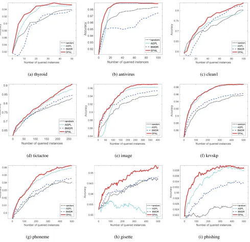
Figure 1: Performance comparison.

Experiments

In this section, we first introduce the compared methods and datasets in the experiments, followed by the implementation settings. Then we illustrate and analyze the performance com-parison results with other methods. Finally, the experiment with different ratios of initially labeled data is performed to examine the robustness of our method.

Settings

To validate the effectiveness of our approach, we conduct experiments to compare the following methods:

• ASPL:Select a batch of most uncertain instances to query and a batch of high confidence samples to assign pseudo-labels (Lin et al. 2018).

• BMDR:Select a batch of informative and representative instances by optimizing the ERM risk bound for active learning (Wang and Ye 2013).

• Random:Select a batch of instances randomly. • SPAL:The method proposed in this paper.

(6)

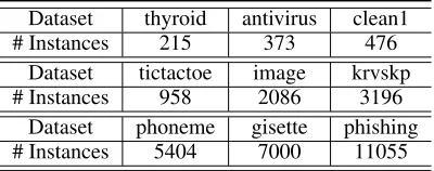
Table 1: Datasets used in the experiments.

Dataset thyroid antivirus clean1

# Instances 215 373 476

Dataset tictactoe image krvskp

# Instances 958 2086 3196

Dataset phoneme gisette phishing # Instances 5404 7000 11055

sample 40% instances as the test set, and the rest 60% in-stances for the training. Further, 5% of the training set is used as the initially labeled data, while the rest instances consist of the unlabeled pool for active selection. The data partition is repeated randomly for 10 times. We fix batch sizeb= 5 for all methods.

Note that the ASPL will add two batches of instances into

Lin each iteration, with half from querying and half from prediction. This causes that the end point of ASPL is earlier than others. Thus we also stop other methods to ensure the numbers of queried instances are the same. For the relatively large datasets, we report the performances of early stage to demonstrate that at a specific training stage, over-complex examples may be less useful than easy ones for improving the model. It is thus important to query the right thing at the right time.

The parameters of BMDR are set to the recommended values in their paper. Specifically, the regularized weight

γ = 0.1and the trade-off parameterµ= 1000. For ASPL, it targets for specific application and can not be applied to binary classification problem directly, so we simplify it to select two batches of samples with the same batch size, one is the most uncertain instances for querying and the other is the most confident instances for assigning predicted labels. For the proposed method SPAL, we fixµ= 0.1, andγ= 0.1. For the SPL parameterλ, we initialize it with a certain value which is selected from{0.1,0.01}, and follow the method used in (Lin et al. 2018) to update it linearly with a small fixed value. In our experiments, we fixλpace= 0.01for all

datasets. Specifically, we have the following updating rule forλattth iteration:

λt=λinitial+ (t−1)∗λpace.

CVX (Grant and Boyd 2014) and MOSEK1_{are used to}

solve the QP problem. We follow (Wang and Ye 2013) to employ a regularized linear model to implement the classifi-cation model for all methods.

Performance comparison

We plot the average accuracy curves of the proposed SPAL and compared methods with queried instances increasing in Figure 1. To further validate the significance of our method, we also conduct paired t-tests at 95 percent significance level when 20%, 40%, 60%, 80%, 100% of the preset number of queries is reached. We present the win/tie/loss counts of SPAL versus the other methods in Table 2.

1

http://www.mosek.com/

Table 2: Win/Tie/Loss counts of SPAL versus the other meth-ods with 20%, 40%, 60%, 80%, 100% of the preset number of queries based on paired t-tests at 95 percent significance level.

Dataset SPAL versus In All

Random BMDR ASPL

thyroid 4/1/0 5/0/0 2/3/0 11/4/0 antivirus 4/1/0 5/0/0 0/5/0 9/6/0

clean1 4/1/0 1/4/0 3/2/0 8/7/0 tictactoe 4/1/0 4/1/0 1/4/0 9/6/0 image 4/1/0 4/1/0 4/1/0 12/3/0 krvskp 5/0/0 5/0/0 2/3/0 12/3/0 phoneme 5/0/0 4/1/0 0/5/0 9/6/0

gisette 5/0/0 3/2/0 5/0/0 13/2/0 phishing 5/0/0 5/0/0 1/4/0 11/4/0 In All 40/5/0 36/9/0 18/27/0 94/41/0

It can be observed from the figure that the proposed SPAL approach outperforms the other methods in most cases. When comparing with BMDR, our method is always superior. It implies that considering the easiness of the instances can save the labeling cost by filtering out instances that are over com-plex for the classification model. ASPL works well on some datasets but fails on the others. Note that in addition to the queried instances, ASPL also adds a batch of instances with predicted labels. That is why its performance is less stable. Because the predicted labels could be unreliable when the model is not well trained. As expected, the random strategy is usually the worst one.

Table 2 shows that our method can outperform the base-line methods significantly in most cases. Note that, although ASPL achieves better performance than random and BMDR by using extra self-annotated instances in model training, it still has the risk that the labeled instances may not be fully utilized by the model. We believe this is the reason why our method can outperform the others.

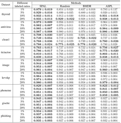
Study on different initially labeled ratios

In this subsection, we further perform the experiments with different ratios of initially labeled data to examine the perfor-mances of compared approaches. Specifically, we compare the methods when the 1%, 5%, 10% and 20% of the training set is initially labeled while other settings remain unchanged. Because of the space limitation, we report the average value of the accuracy curve instead of plotting the whole curve. For each case, the best result and its comparable performances are highlighted in boldface based on paired t-tests at 95 per-cent significance level. The mean and standard deviation of accuracies are presented in Table 3.

(7)

Table 3: Influence of different initially labeled ratios (mean±std). The best performance and its comparable performances based on paired t-tests at 95 percent significance level are highlighted in boldface.

Dataset Different labeled ratios

Methods

SPAL Random BMDR ASPL

thyroid

1% 0.879±0.019 0.854±0.020 0.837±0.016 0.783±0.137 5% 0.929±0.016 0.899±0.035 0.889±0.032 0.920±0.015 10% 0.933±0.014 0.913±0.030 0.916±0.023 0.931±0.018

20% 0.935±0.013 0.929±0.022 0.928±0.015 0.938±0.013

antivirus

1% 0.973±0.009 0.956±0.013 0.921±0.025 0.964±0.009 5% 0.982±0.007 0.970±0.011 0.954±0.017 0.978±0.008 10% 0.985±0.007 0.976±0.012 0.963±0.018 0.984±0.009

20% 0.987±0.008 0.980±0.011 0.976±0.013 0.986±0.008

clean1

1% 0.708±0.030 0.687±0.031 0.681±0.025 0.654±0.026 5% 0.749±0.034 0.719±0.032 0.725±0.022 0.727±0.038 10% 0.768±0.036 0.742±0.029 0.739±0.028 0.760±0.026

20% 0.788±0.024 0.775±0.025 0.776±0.020 0.780±0.028

tictactoe

1% 0.763±0.013 0.727±0.019 0.722±0.024 0.756±0.027

5% 0.786±0.017 0.748±0.021 0.761±0.022 0.775±0.020

10% 0.810±0.015 0.766±0.024 0.749±0.027 0.803±0.011

20% 0.839±0.010 0.794±0.027 0.769±0.028 0.838±0.013

image

1% 0.933±0.007 0.896±0.011 0.916±0.007 0.909±0.013 5% 0.944±0.008 0.916±0.009 0.929±0.006 0.933±0.010 10% 0.953±0.007 0.928±0.009 0.938±0.005 0.949±0.007 20% 0.961±0.004 0.941±0.007 0.947±0.004 0.960±0.005

krvskp

1% 0.942±0.004 0.899±0.012 0.910±0.005 0.936±0.003 5% 0.964±0.004 0.928±0.010 0.937±0.006 0.962±0.004 10% 0.974±0.004 0.943±0.009 0.949±0.008 0.972±0.004 20% 0.980±0.003 0.956±0.006 0.958±0.006 0.979±0.004

phoneme

1% 0.829±0.007 0.808±0.008 0.812±0.009 0.823±0.012

5% 0.844±0.008 0.826±0.008 0.829±0.006 0.841±0.007

10% 0.851±0.004 0.837±0.007 0.838±0.008 0.850±0.005

20% 0.861±0.006 0.845±0.007 0.845±0.007 0.859±0.005

gisette

1% 0.945±0.003 0.930±0.005 0.931±0.005 0.927±0.003 5% 0.947±0.003 0.942±0.004 0.943±0.005 0.933±0.005 10% 0.951±0.004 0.946±0.004 0.947±0.003 0.935±0.003 20% 0.952±0.003 0.950±0.003 0.950±0.004 0.938±0.003

phishing

1% 0.934±0.003 0.919±0.007 0.918±0.006 0.931±0.002 5% 0.937±0.003 0.924±0.009 0.930±0.004 0.935±0.003 10% 0.936±0.003 0.925±0.008 0.926±0.008 0.934±0.003 20% 0.935±0.003 0.927±0.006 0.927±0.007 0.932±0.004

the other approaches, because it adds two batches with one from querying and one from prediction. When there is more labeled data, the model prediction is more reliable, and thus ASPL can benefit more from the extra pseudo labels. For BMDR, its performance is still worse than ours even in dif-ferent initial ratios of labeled data which implies that it is important to further consider the easiness of instances even they have high potential value.

In addition, we also observe some trends in the table that the proposed method SPAL favors the case with less labeled data. One possible reason is that many examples are over-difficult for a simple model, and thus we need a self-paced strategy to select the easy ones at such an early learning stage to get cost-effective queries. We believe this is an advantage because active learning is especially important when labeled

data is limited.

Conclusion

(8)

References

Basu, S., and Christensen, J. 2013. Teaching classification boundaries to humans. In Proceedings of the 27th AAAI Conference on Artificial Intelligence.

Bengio, Y.; Louradour, J.; Collobert, R.; and Weston, J. 2009. Curriculum learning. In Proceedings of the 26th Annual International Conference on Machine Learning, 41–48. Bezdek, J. C., and Hathaway, R. J. 2003. Convergence of alternating optimization. Neural, Parallel, and Scientific Computations11(4):351–368.

Borgwardt, K. M.; Gretton, A.; Rasch, M. J.; Kriegel, H.; Sch¨olkopf, B.; and Smola, A. J. 2006. Integrating structured biological data by kernel maximum mean discrepancy. In Proceedings 14th International Conference on Intelligent Systems for Molecular Biology, 49–57.

Boyd, S. P.; Parikh, N.; Chu, E.; Peleato, B.; and Eckstein, J. 2011. Distributed optimization and statistical learning via the alternating direction method of multipliers.Foundations and Trends in Machine Learning3(1):1–122.

Chattopadhyay, R.; Wang, Z.; Fan, W.; Davidson, I.; Pan-chanathan, S.; and Ye, J. 2012. Batch mode active sampling based on marginal probability distribution matching. InThe 18th ACM SIGKDD International Conference on Knowledge Discovery and Data Mining, 741–749.

Dasgupta, S., and Hsu, D. J. 2008. Hierarchical sampling for active learning. InProceedings of the 15th International Conference on Machine Learning, 208–215.

Grant, M., and Boyd, S. 2014. CVX: Matlab software for disciplined convex programming, version 2.1. http://cvxr. com/cvx.

Gretton, A.; Borgwardt, K. M.; Rasch, M. J.; Sch¨olkopf, B.; and Smola, A. J. 2006. A kernel method for the two-sample-problem. In Advances in Neural Information Processing Systems, 513–520.

Hoi, S. C. H.; Jin, R.; Zhu, J.; and Lyu, M. R. 2008. Semi-supervised SVM batch mode active learning for image re-trieval. InIEEE Conference on Computer Vision and Pattern Recognition.

Huang, S., and Zhou, Z. 2013. Active query driven by uncertainty and diversity for incremental multi-label learn-ing. InIEEE 13th International Conference on Data Mining, 1079–1084.

Huang, S.; Jin, R.; and Zhou, Z. 2014. Active learning by querying informative and representative examples. IEEE Transactions on Pattern Analysis and Machine Intelligence 36(10):1936–1949.

Jiang, L.; Meng, D.; Mitamura, T.; and Hauptmann, A. G. 2014. Easy samples first: Self-paced reranking for zero-example multimedia search. In Proceedings of the ACM International Conference on Multimedia, 547–556.

Khan, F.; Mutlu, B.; and Zhu, X. 2011. How do humans teach: On curriculum learning and teaching dimension. InAdvances in Neural Information Processing Systems, 1449–1457. Kumar, M. P.; Packer, B.; and Koller, D. 2010. Self-paced learning for latent variable models. InAdvances in Neural Information Processing Systems, 1189–1197.

Lee, Y. J., and Grauman, K. 2011. Learning the easy things first: Self-paced visual category discovery. InThe 24th IEEE Conference on Computer Vision and Pattern Recognition, 1721–1728.

Lin, L.; Wang, K.; Meng, D.; Zuo, W.; and Zhang, L. 2018. Active self-paced learning for cost-effective and progressive face identification. IEEE Transactions on Pattern Analysis and Machine Intelligence40(1):7–19.

Ma, F.; Meng, D.; Xie, Q.; Li, Z.; and Dong, X. 2017. Self-paced co-training. InProceedings of the 34th International Conference on Machine Learning, 2275–2284.

Settles, B. 2009. Active learning literature survey. Technical report, University of Wisconsin-Madison.

Seung, H. S.; Opper, M.; and Sompolinsky, H. 1992. Query by committee. InProceedings of the 5th Annual Workshop on Computational Learning Theory, 287–294.

Supancic, J. S., and Ramanan, D. 2013. Self-paced learn-ing for long-term tracklearn-ing. In2013 IEEE Conference on Computer Vision and Pattern Recognition, 2379–2386. Tang, J.; Zha, Z.; Tao, D.; and Chua, T. 2012. Semantic-gap-oriented active learning for multilabel image annotation. IEEE Transactions on Image Processing21(4):2354–2360. Tang, Y.; Yang, Y.; and Gao, Y. 2012. Self-paced dictionary learning for image classification. InProceedings of the 20th ACM Multimedia Conference, 833–836.

Wang, Z., and Ye, J. 2013. Querying discriminative and representative samples for batch mode active learning. InThe 19th ACM SIGKDD International Conference on Knowledge Discovery and Data Mining, 158–166.

Wang, K.; Wang, Y.; Zhao, Q.; Meng, D.; and Xu, Z. 2017. SPLBoost: An improved robust boosting algorithm based on self-paced learning.arXiv preprint arXiv:1706.06341. Xu, C.; Tao, D.; and Xu, C. 2015. Multi-view self-paced learning for clustering. InProceedings of the 24th Interna-tional Joint Conference on Artificial Intelligence, 3974–3980. Yan, Y., and Huang, S. 2018. Cost-effective active learning for hierarchical multi-label classification. InProceedings of the27th International Joint Conference on Artificial Intelli-gence, 2962–2968.

Zhang, D.; Meng, D.; Zhao, L.; and Han, J. 2016. Bridg-ing saliency detection to weakly supervised object detection based on self-paced curriculum learning. InProceedings of the 25th International Joint Conference on Artificial Intelli-gence, 3538–3544.

Zhang, D.; Meng, D.; and Han, J. 2017. Co-saliency detection via a self-paced multiple-instance learning framework.IEEE Transactions on Pattern Analysis and Machine Intelligence 39(5):865–878.