Oversampling for Imbalanced Data via Optimal Transport

(1)

The Thirty-Third AAAI Conference on Artificial Intelligence (AAAI-19)

Oversampling for Imbalanced Data via Optimal Transport

Yuguang Yan,

1,2∗†

Mingkui Tan,

1∗

Yanwu Xu,

3∗

Jiezhang Cao,

1

Michael Ng,

4

Huaqing Min,

1

Qingyao Wu

1‡ 1_{School of Software Engineering, South China University of Technology, China}

2_{CVTE Research, Guangzhou Shiyuan Electronics Co., Ltd., China} 3_{Artificial Intelligence Innovation Business, Baidu Inc., China}

4_{Department of Mathematics, Hong Kong Baptist University, Hong Kong, China}

{yan.yuguang,secaojiezhang}@mail.scut.edu.cn,{mingkuitan,qyw,hqmin}@scut.edu.cn, [email protected], [email protected]

Abstract

The issue of data imbalance occurs in many real-world appli-cations especially in medical diagnosis, where normal cases are usually much more than the abnormal cases. To alleviate this issue, one of the most important approaches is the over-sampling method, which seeks to synthesize minority class samples to balance the numbers of different classes. How-ever, existing methods barely consider global geometric in-formation involved in the distribution of minority class sam-ples, and thus may incur distribution mismatching between real and synthetic samples. In this paper, relying on optimal transport (Villani 2008), we propose an oversampling method by exploiting global geometric information of data to make synthetic samples follow a similar distribution to that of mi-nority class samples. Moreover, we introduce a novel regu-larization based on synthetic samples and shift the distribu-tion of minority class samples according to loss informadistribu-tion. Experiments on toy and real-world data sets demonstrate the efficacy of our proposed method in terms of multiple metrics.

Introduction

The imbalanced data issue occurs in many real-world ap-plications, where the samples of one class are much more than samples of other classes (He and Garcia 2008; Branco, Torgo, and Ribeiro 2016; Lin et al. 2018; Gonz´alez et al. 2019). Especially in the area of medical diagnosis, the ab-normal samples with a disease are expensive and difficult to collect, while normal samples are much easier to obtain. As a result, we usually face an imbalanced learning prob-lem where normal samples are much more than the abnor-mal ones (Bhattacharya, Rajan, and Shrivastava 2017).

Standard machine learning methods usually focus on re-ducing loss over the whole training data set. These meth-ods usually pay more attention to the training loss on ma-jority class samples while omitting the minority class sam-ples, thus fail to achieve promising performance. This issue

∗

The co-first author. †

This work was done when Yuguang Yan was an intern at Med-ical Image and Signal Processing Group, CVTE Research.

‡

The corresponding author.

becomes even worse in medical diagnosis, since misclassi-fying an abnormal one is much severer than misclassimisclassi-fying a normal one, which will delay the medical treatment.

To alleviate the imbalanced issue, several kinds of algo-rithms have been proposed in the last decades. Among these methods, oversampling attracts much attention because of its simplicity and efficacy (Fern´andez et al. 2018). Oversam-pling aims to synthesize minority class samples to balance the numbers of different classes, so that standard machine learning methods can be performed on the augmented data set. Oversampling methods usually synthesize new samples based on a minority class sample and its nearest neighbors. However, they barely consider global geometric information in the distribution of minority class samples, and thus may incur distribution mismatching between real and synthetic samples obtained by oversampling methods.

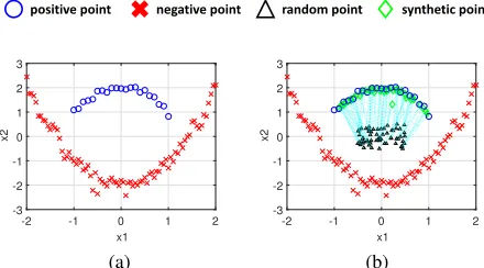
In this paper, we aim to exploit global geometric infor-mation of data to oversample minority class samples via op-timal transport (Villani 2008). Motivated by this, we pro-pose a novel oversampling method calledOptimalTransport forOverSampling (OTOS), which applies optimal transport to synthesize samples that follow a similar distribution to the one of minority class samples. Specifically, we move random points from a prior distribution to that of minority class samples, as shown in Figure 1, so that the transported samples can be taken as synthetic minority class data for training. In addition, we introduce a regularization based on the transported samples for optimal transport, and leverage loss information to concentrate more on those minority class samples close to the decision boundary.

We apply a projected gradient method to optimize the re-sultant constrained problem, and conduct extensive experi-ments on both toy and real-world data sets, including bench-mark data from LIBSVM1 and medical image data. Mul-tiple metrics regarding imbalanced learning are adopted to demonstrate the effectiveness of our proposed method.

The principal contributions are summarized as follows: • We exploit global geometric information of data via

opti-mal transport to guarantee distribution matching between synthetic and real minority class samples.

1

(2)

positive point negative point random point synthetic point

-2 -1 0 1 2 x1

-3 -2 -1 0 1 2 3

x2

(a)

-2 -1 0 1 2 x1

-3 -2 -1 0 1 2 3

x2

(b)

Figure 1: An illustration of our idea. Positive and neg-ative points are minority and majority class samples, re-spectively. (a) Positive points and negative points. (b) Pos-itive points, negative points, random points, and synthetic points obtained by optimal transport. Dot lines indicate the transport plan from random points to synthetic points, and random points are drawn from the uniform distribution U(−0.5,0.5).

• We shift the empirical distribution of minority class sam-ples based on training loss, rather than adopting a uniform distribution for them, which is commonly used in existing works (Courty et al. 2017b; Yan et al. 2018).

• We design a novel regularization with transported samples to avoid synthesizing noisy samples, which is achieved by enlarging the difference between the predicted values of a transported sample and a majority class sample.

Related Studies

Imbalanced Learning

Most existing methods of imbalanced learning belong to two categories: cost-sensitive approaches and oversampling approaches (Lemaˆıtre, Nogueira, and Aridas 2017). Cost-sensitive approaches try to assign different weights for classes, so that losses on minority class samples are em-phasized to contribute more for training (Liu et al. 2017; Zhang et al. 2018). Nevertheless, these methods omit geo-metric information hidden in the structure of training data, which limits their performance on imbalanced problems.

Oversampling approaches seek to augment minority class data to balance the numbers of two classes (Das, Krishnan, and Cook 2015; Sen et al. 2016; Abdi and Hashemi 2016; P´erez-Ortiz et al. 2016; Bellinger, Drummond, and Japkow-icz 2018). Among them, SMOTE is a classical method, which takes linear interpolations of a minority class sample and its nearest neighbors as new training samples (Chawla et al. 2002). bSMOTE improves SMOTE by finding so-called DANGER samples from the minority class (Han, Wang, and Mao 2005). ADASYN further extends SMOTE by consid-ering different effects of training samples (He et al. 2008). In (Das, Krishnan, and Cook 2015), a Gibbs oversampling method is proposed. MWMOTE finds informative minority class samples and oversample data based on a clustering ap-proach (Barua et al. 2014). (Peng 2015) proposes an

adap-tive sampling method to form multiple classifiers over dif-ferent subsets. (Fern´andez et al. 2018) provides a summary regarding recent advances of SMOTE.

Compared to the above oversampling methods, the key differences in our work are two folds: firstly, we exploit global geometric information of data via optimal transport, which makes synthetic samples follow a similar distribution to that of minority class samples, while existing oversam-pling methods barely consider the global geometric infor-mation; secondly, our proposed method provides a global oversampling paradigm based on the Wasserstein barycen-ter (Cuturi and Doucet 2014; Peyr´e and Cuturi 2017), which does not rely on nearest neighbor searching commonly used in existing oversampling methods.

Optimal Transport

Optimal transport (Villani 2008), which was firstly intro-duced by Monge in (Monge 1781), originally aims to study how to transport mass into a given place with the mini-mal cost. After that, Kantorovitch further developed opti-mal transport and applied it for economic applications (Kan-torovitch 1958). The minimal cost in optimal transport is also known as the Wasserstein distance or Earth Mover Dis-tance. To efficiently solve the optimization problem involved in optimal transport, some fast numerical algorithms are pro-posed in (Cuturi 2013; Benamou et al. 2015). Recently, opti-mal transport has been actively applied in machine learning problems (Peyr´e and Cuturi 2017). In (Courty et al. 2017a; 2017b), optimal transport is applied in unsupervised domain adaptation. Yan et al. leveraged optimal transport to address the problem of heterogeneous domain adaptation in (Yan et al. 2018). The Wasserstein distance is also used in the gen-erative model to measure the distance between two distribu-tions (Arjovsky, Chintala, and Bottou 2017).

Methodology

Problem Statement and Notations

Given training dataX = [x1, . . . ,xn]> ∈ Rn×dand their

labels y = [y1, . . . , yn]> ∈ {+1,−1}n, where n is the

number of training data, and d is the number of features. Among the training data, the positive data are represented as X+_{= [}_x+

1, . . . ,x +

n+]

>_∈ Rn

+_×_d

withn+_{being the number}

of positive samples, and the negative data are represented as X− _{= [}_x−

1, . . . ,x

−

n−]> ∈ Rn −

×d _with_n−_{being the}

num-ber of negative samples. Without loss of generality, we have

n+ _n−_{, which means that the number of positive}

sam-ples is much smaller than that of negative samsam-ples. We also call the positive label as the minority class, and the negative label as the majority class.

1ndenotes a vector in the spaceRnwith all the elements

being 1. For a vectora, diag(a)is a diagonal matrix with the diagonal elements being a. For a matrixA, letAij be

the(i, j)-th element ofA. The trace of the square matrixA is defined as tr(A) =P

iAii.For two matricesAandB, let

A⊗Bbe the Kronecker product,ABbe the element-wise product, and the inner product is defines as

hA,Bi=X

i

X

j

(3)

Optimal Transport for Oversampling

Optimal transport aims to transport samples from one dis-tribution to another disdis-tribution with the minimal transport cost (Peyr´e and Cuturi 2017; Courty et al. 2017b). As a re-sult, we can obtain more samples in the target distribution. Motivated by this, we apply optimal transport to transport some random samples into the distribution of minority class samples to augment training data.

Specifically, letµrbe the empirical distributions of a set of random vectors{xr

i}n

r

i=1drawn from a prior distribution,

andµ+ _{be the empirical distribution of positive samples,}

which are minority class samples in this paper. We propose to transport samples fromµr_into_µ+ _{to augment positive}

samples. Define δ be the Dirac function at one point, pr_i

andp+_i be probability masses with the simplex constraints

Pnr

i=1p

r

i = 1and

Pn+

i=1p +

i = 1. The two empirical

distri-butions are written as

µr=

nr

X

i=1

pr_iδr_i, µ+=

n+ X

i=1

p+_i δ_i+. (1)

A transport plan is represented as a joint distribution, which is in the following definition domain:

T ={T∈(_R+)nr×n+|T1n+=µr,T>1nr =µ+}, (2) and the entropy ofTis defined as

H(T) =−X

ij

Tij(logTij−1).

Optimal transport aims to find a transport matrix with the minimal cost, which is modelled as the following optimiza-tion problem:

min T∈T hT,C

r+

i −H(T), (3)

whereis a trade-off parameter,Cr+_{is the cost matrix with} C_ijr+being defined as

C_ijr+=c(xri,x

+

j) =kx r i −x

+

jk

2

2, (4)

and the entropic regularization H(T)is used to smoothen the solution and speed up the optimization (Cuturi 2013). In this way, the transported samples follow a similar distri-bution to that of positive samples and can be taken as aug-mented positive data. Specifically, letnr₌_n−₋_n+_{, so the}

numbers of samples from two classes are balanced.

Oversampling by Data Transport

After obtaining the optimal transport matrixT, we can trans-port the random vectors into the distribution of the positive samples based on the Wasserstein barycenter, which repre-sents the random points in the distribution of positive data (Cuturi and Doucet 2014; Peyr´e and Cuturi 2017). Specifi-cally, for the pointxr

i, its representation in the positive data

distribution is denoted byxˆr

i, which is obtained by solving

the following optimization problem:

ˆ

xr_i = arg min x∈Rd

X

j

Tijc(x,x+j)

= arg min x∈Rd

X

j

Tijkx−x+jk

2 2.

(5)

Taking the partial derivativew.r.t.xto zero, we obtain

X

j

Tijx−

X

j

Tijx+j =0, (6)

and the solution is given by the following:

ˆ xri =

P

jTijx+j

P

jTij

. (7)

Based on this, the transported data matrix can be written as

ˆ

X=diag(T1n+)−1TX+=diag(µr)−1TX+. (8)

For simplicity, defineDr=diag(µr)−1, and Eq. (8) can be

rewritten as

ˆ

X=DrTX+. (9)

From Eq. (9), we observe that each synthetic positive sam-ple is a convex combination of multisam-ple positive samsam-ples. This indicates that our approach leverages global informa-tion from all the given minority class samples, which differs from nearest neighbor searching commonly used in existing oversampling methods. Therefore, global geometric infor-mation extracted from minority class samples are exploited in our approach.

Distribution Shifting based on Training Loss

Forµr, we simply adopt a uniform distribution,i.e.,µr = [_n1r, . . . ,

1

nr]

>_{. For}_µ+_{, without more information about the}

underlying distribution of positive data, one usually adopts a uniform distribution (Courty et al. 2017b; Yan et al. 2018),

i.e., µ+ _{= [} 1

n+, . . . ,

1

n+]>, in Problem (3). However, this approach omits the loss information of samples. For SVM, a sample closer to the decision boundary usually has a larger loss and more information than one far away from the deci-sion boundary.

Motivated by this intuition, we firstly pretrain an SVM classifier, and then shift the positive data distribution based on training loss to concentrate more on the ones with larger loss values. Formally, we pretrain an SVM classifier with the hinge loss, which is given as

min w,ξ

1 2kwk

2 2+C

n

X

i=1 ξi

s.t. yiw>xi≥1−ξi, ξi≥0, i= 1, . . . , n,

(10)

where C is the trade-off parameter for loss. Let ξ_i+ = max(1−y+_i w>x+_i ,0)be the hinge loss of the positive sam-plex+_i , we apply the softmax function to shift the distribu-tion of{x+_i }n+

i=1as

µ+=h e

ξ+₁

Pn+

i=1eξ

+ i

, . . . , e

ξ+ n₊

Pn+

i=1eξ

+ i

i>

. (11)

(4)

Learning with Transported Samples

Concentrating on those samples close to the decision bound-ary can take better advantage of training samples. However, a potential issue is that a few minority class samples that are close to majority class samples may highly affect the results of optimal transport, making some transported samples too close to majority class samples and confusing the training of the classifier. This issue will become even severer with noisy minority samples. In order to alleviate this, for each pair of a transported positive sample and a negative sample, we propose to enlarge the difference between the predicted values of them obtained by the pretrained model. To achieve this, we design the following regularization:

Ω(T) = 1 2

nr

X

i=1

n−

X

j=1 w

>_x_ˆ

i−w>x−j

−1 2

, (12)

and seek to solve the optimization problem as

min

T∈T L(T),Ω(T) +λhT,C

r+_{i −}_H₍_T₎_,

(13)

whereλandare trade-off parameters. By rearranging the above objective function, we obtain

L(T) = 1 2

nr

X

i=1 n−

X

j=1

w

>

ˆ

xi−w

>

x−j

−1

2

+λtr(T>Cr+)−H(T)

= 1 2n

− tr

ˆ

Xww>Xˆ>−n−tr

ˆ

X(1>nr⊗w)

−trX 1ˆ >nr⊗(ww>(X−)>1_n−)

+λtr(T>Cr+)−H(T) +constant.

(14)

By substituting Eq. (9) into Eq. (14), we simplifyL(T)as

L(T) =1 2n

− tr

DrTX+ww>(X+)>T>D>r

−trDrTX+ 1

>

nr⊗((ww>(X−)>1_n−) +n−w)

+λtr(T>Cr+)−H(T) +constant

=1 2n

−

trTX+ww>(X+)>T>D>rDr

−trTX+ 1>nr⊗((ww>(X−)>1_n−) +n−w)Dr

+λtr(T>Cr+)−H(T) +constant.

(15)

We define the matrix variablesΘ,ΦandΨas

Θ=λ(Cr+)>−X+ 1>nr⊗((ww>(X−)>1_n−) +n−w)Dr,

Φ=X+ww>(X+)>,

Ψ=D>rDr.

(16)

As a result,L(T)is reformulated as

L(T) = 1 2n

−_tr_TΦT>_Ψ₊_tr₍_TΘ₎₋_H₍_T_{) +}_constant_.

(17)

Optimization Details

For simplicity, we define

f(T) =1 2n

−_tr_TΦT>_Ψ₊_tr₍_TΘ₎_, ₍₁₈₎

andL(T)can be rewritten as

L(T) =f(T)−H(T) +constant. (19)

Minimizing L(T)w.r.t. T is non-trivial because of the equality constraints. To solve it, we apply a projected gra-dient descent algorithm based on the exponentiated gragra-dient and the Kullback-Leibler divergence (Benamou et al. 2015; Peyr´e, Cuturi, and Solomon 2016). Specifically, at theτ-th iteration, we firstly updateTτby the exponentiated gradient

method as follows:

˜

Tτ :=Tτexp

−α∇L(Tτ)

, (20)

whereα > 0 is a step size. After that, we projectT˜τ into

the definition domainT with the Kullback-Leibler metric as

Tτ+1:= ΠKLT ( ˜Tτ) = arg min

T0_∈T

KL(T0|T˜τ). (21)

According to (Benamou et al. 2015), the projection opera-tion in Eq. (21) can be rewritten as the following regularized optimal transport problem:

Tτ+1 := ΠKLT ( ˜Tτ)

= arg min T0_∈T

h−log( ˜Tτ),T0i −H(T0),

(22)

which can be efficiently solved by the Sinkhorn’s fixed point algorithm (Sinkhorn 1967; Cuturi 2013). In Problem (22), the transport cost matrix−log( ˜Tτ)can be simplified as

−log( ˜Tτ) =−log

Tτexp −α∇L(Tτ)

=∇f(Tτ)

=Θ>+n−ΨTτΦ,

(23)

where we setα= 1.

Algorithm 1 summarizes the procedure of OTOS.

Algorithm 1Optimal Transport for OverSampling (OTOS)

1: InitializeT=µr₍_µ+₎>_,_τ _{= 1}_.

2: TrainwoverX+_and_X−_{by solving Problem (10).}

3: Computeµ+based on Eq. (11).

4: ConstructΘ,ΦandΨaccording to Eq. (16). 5: repeat

6: Calculate Eq. (23) based onTτ.

7: ObtainTτ+1by solving Problem (22).

8: τ:=τ+ 1. 9: untilConvergence.

(5)

positive point negative point random point synthetic point

-2 -1 0 1 2 x1

-1 0 1 2 3

x2

(a)

-2 -1 0 1 2 x1

-1 0 1 2 3

x2

(b)

-2 -1 0 1 2 x1

-1 0 1 2 3

x2

(c)

-2 -1 0 1 2 x1

-1 0 1 2 3

x2

(d)

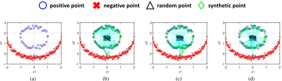
Figure 2: Results on a 2D toy data set. Positive and negative points are minority and majority class samples, respectively. (a) Positive points and negative points. (b) Positive points, negative points, and synthetic points obtained by OTOS-α. (c) Positive points, negative points, and synthetic points obtained by OTOS-β. (d) Positive points, negative points, and synthetic points obtained by OTOS. Dot lines indicate the transport plan from random points to synthetic points.

Experiments

To verify our proposed method, we firstly conduct empirical studies on a toy data set, and then apply our method on sev-eral real-world data sets, which include benchmark data sets from LIBSVM and medical image data.

Compared Methods

• SVM. We perform SVM (Fan et al. 2008) on an imbal-anced data set to train a classifier. SVM is a straightfor-ward method without considering the imbalance issue. • ROS. Random oversampling (ROS) randomly selects

samples from the minority class and adds them to train-ing data.

• SMOTE. In the method of synthetic minority oversam-pling technique (SMOTE) (Chawla et al. 2002), for a mi-nority class sample, the linear interpolations of it and its nearest neighbors are taken as new samples for training. • bSMOTE. Borderline-SMOTE (bSMOTE) (Han, Wang,

and Mao 2005) firstly finds some so-called DANGER samples for the minority class, and then takes the linear interpolations of them and their nearest neighbors as new training samples.

• ADASYN. Adaptive synthetic (ADASYN) (He et al. 2008) extends SMOTE by adaptively adjusting the num-bers of artificial samples for each minority class sample. If a minority class sample has more nearest neighbors be-longing to the majority class, ADASYN will synthesize more artificial samples based on the sample and its near-est neighbors.

• MWMOTE. Majority weighted minority oversampling technique (MWMOTE) (Barua et al. 2014) identifies in-formative minority class samples, and synthesizes sam-ples according to the weighted informative minority class samples based on a clustering method.

• OTOS-α. OTOS-α is a simplified version of OTOS. OTOS-αadopts a uniform distribution forµ+. It firstly obtainsTby solving Problem (3), and then synthesizes samples based on Eq. (9).

• OTOS-β. OTOS-βis also a simplified version of OTOS. OTOS-β replaces the uniform distribution of µ+ _in

OTOS-α by the distribution in Eq. (11).

Experiments on Toy Data

To demonstrate the effects of the proposed method, we firstly conduct experiments on a 2D toy data set, in which 42 positive points are minority class samples, and 201 nega-tive points are majority class samples. Figure 2(a) shows the positive and negative points.

From Figure 2(b), the synthetic points obtained by

OTOS-αfollow a similar distribution to that of the minority class samples. Figure 2(c) presents synthetic points obtained by OTOS-β. Compared to OTOS-α, OTOS-βsynthesizes more samples near to those samples that are close to the borderline between two classes, since it pays more attention to those samples based on the distribution in Eq. (11). Nevertheless, the nearest positive point to the negative ones highly affects the result of OTOS-β, making it sensitive to noisy samples. Figure 2(d) shows the results of OTOS. Compared to

OTOS-α, OTOS synthesizes more samples close to the borderline between two classes. In addition, by introducing the regu-larization in Eq. (12) into optimal transport, OTOS is more robust to noisy points than OTOS-β.

Experiments on Real-World Data

Data Sets Tables 1 and 2 present the statistical informa-tion of the adopted benchmark and medical image data sets, respectively. In the tables, “size” represents #samples× #f eatures, and “ratio” is #_#majority class samples_{minority class samples}. In the following, we describe the details of the data sets.

(6)

Table 1: Statistical information of the benchmark data sets.

name size ratio australian 690×14 1.25 breast-cancer 683×10 1.86 diabetes 768×8 1.87 german 1,000×24 2.33 svmguide2 391×20 1.30 svmguide4 300×10 4.66

Table 2: Statistical information of the medical image data sets.

name size ratio

ORIGA 650×2,048 2.87 iSee-AMD 8,480×2,048 10.78

iSee-DR 8,016×2,048 30.31 iSee-glaucoma 8,208×2,048 17.32

• Medical data. We also use four fundus image data sets, among which iSee-AMD, iSee-DR, iSee-glaucoma are used to detect Age-Related Macular Degeneration (AMD), Diabetic Retinopathy (DR) and glaucoma, re-spectively, and ORIGA is used to detect glaucoma. We ex-tract features from the pool5 layer of the ResNet-152 (He et al. 2016) pretrained on ImageNet (Deng et al. 2009) to obtain a 2,048-dimensional vector for one image.

Experimental Settings For all the compared methods, we synthesize minority class samples until that the numbers of minority and majority class samples are the same, and use linear SVM with the default parameterC= 1as the classi-fier. For our method, we draw random samples from a prior uniform distributionU(0,1). The parametersλandare se-lected in the range10{−1,0,1,2,3,4,5}_{, and the best results are}

adopted. We repeat all the experiments 10 times and report the mean and standard derivation values, and results of each time are obtained by the mean of 10-fold cross-validation.

Evaluation Metrics We adopt multiple evaluation metrics to test the performance of the proposed method. Specifically, letyi be a true label andyˆibe a predicted label, we count

the numbers of true positive (T P), false positive (F P), false negative (F N) and true negative (T N) samples, which are formally defined as follows:

T P ={xi|yi= +1∧yˆi= +1, i= 1, . . . , n}

,

F P ={xi|yi=−1∧yˆi= +1, i= 1, . . . , n}

,

F N ={xi|yi= +1∧yˆi=−1, i= 1, . . . , n}

,

T N ={xi|yi=−1∧yˆi=−1, i= 1, . . . , n}

.

(24)

Based on the above notations, we define the following met-rics:

Sensitivity= T P

T P +F N, (25)

F1 = 2·T P

2·T P+F N+F P, (26)

G-mean=

r

T P

T P +F N ·

T N

T N+F P. (27)

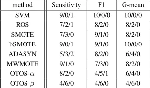
Table 3: Significance test results (win/tie/loss) with paired t-test at 0.05 level for OTOS against other methods.

method Sensitivity F1 G-mean SVM 9/0/1 10/0/0 10/0/0 ROS 7/2/1 8/2/0 8/2/0 SMOTE 7/3/0 9/1/0 8/2/0 bSMOTE 9/0/1 9/1/0 10/0/0 ADASYN 5/3/2 8/2/0 6/4/0 MWMOTE 9/1/0 7/3/0 8/2/0 OTOS-α 8/2/0 4/5/1 6/4/0 OTOS-β 4/6/0 4/6/0 4/6/0

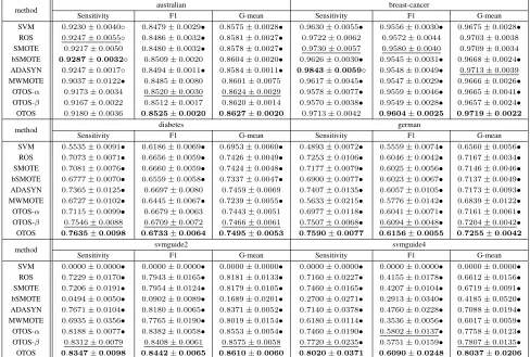
Results and Discussions Table 3 summarizes the signifi-cance test results for OTOS against other methods on all the metrics and adopted data sets, and Tables 4 and 5 present the results on the benchmark and medical image data sets, respectively. The best results are indicated with boldface type and the second best results are underlined. We also apply paired t-test at 0.05 level for performing the signifi-cance tests between OTOS and other methods. “•” means that OTOS significantly outperforms a baseline method, and “◦” means that a baseline method significantly outperforms OTOS. We draw several interesting observations as follows. • OTOS achieves the best Sensitivity results on 7 data sets, the best F1 results on 7 data sets, and the best G-mean results on all the adopted data sets. This demonstrates the effectiveness of OTOS.

• For all the three metrics, most of the best or the second best results are obtained by OTOS-α, OTOS-β or OTOS, which indicates that optimal transport is able to synthe-size high-quality minority class samples to enhance the classification performance.

• Compared to OTOS-αand OTOS-β, OTOS usually gets better or highly comparable results, which verifies the ef-fects of the shifted distribution in Eq. (11) and the regu-larization in Eq. (12).

• OTOS-β performs better than OTOS-αon most exper-iments, which validates that concentrating on minority class samples close to a borderline between two classes is beneficial for training an effective classifier.

• From Table 3, OTOS significantly outperforms other methods on most comparisons, which demonstrates the consistent superiority of OTOS over other methods.

Conclusion

(7)

Table 4: Results on the benchmark data sets.

method australian breast-cancer

Sensitivity F1 G-mean Sensitivity F1 G-mean SVM 0.9230±0.0040◦ 0.8479±0.0029• 0.8575±0.0028• 0.9630±0.0055• 0.9556±0.0030• 0.9675±0.0028•

ROS 0.9247±0.0055◦ 0.8486±0.0032• 0.8581±0.0027• 0.9722±0.0062 0.9572±0.0044 0.9703±0.0038

SMOTE 0.9217±0.0050 0.8480±0.0032• 0.8578±0.0027• 0.9730±0.0057 0.9580±0.0040 0.9709±0.0034

bSMOTE 0.9287±0.0032◦ 0.8509±0.0020 0.8604±0.0020• 0.9626±0.0030• 0.9545±0.0031• 0.9668±0.0024•

ADASYN 0.9247±0.0017◦ 0.8494±0.0011• 0.8584±0.0011• 0.9843±0.0059◦ 0.9548±0.0049• 0.9713±0.0039

MWMOTE 0.9037±0.0122• 0.8485±0.0080 0.8601±0.0075 0.9617±0.0045• 0.9547±0.0029• 0.9666±0.0026•

OTOS-α 0.9173±0.0034 0.8520±0.0030 0.8624±0.0029 0.9578±0.0077• 0.9559±0.0046• 0.9665±0.0041•

OTOS-β 0.9167±0.0022 0.8512±0.0017 0.8620±0.0014 0.9570±0.0038• 0.9549±0.0028• 0.9657±0.0024•

OTOS 0.9180±0.0036 0.8525±0.0020 0.8627±0.0020 0.9713±0.0042 0.9604±0.0025 0.9719±0.0022

method diabetes german

Sensitivity F1 G-mean Sensitivity F1 G-mean SVM 0.5535±0.0091• 0.6186±0.0069• 0.6953±0.0060• 0.4893±0.0072• 0.5559±0.0074• 0.6560±0.0056•

ROS 0.7073±0.0071• 0.6656±0.0059• 0.7426±0.0049• 0.7253±0.0106• 0.6046±0.0042• 0.7167±0.0034•

SMOTE 0.7081±0.0076• 0.6660±0.0059• 0.7424±0.0048• 0.7177±0.0079• 0.6025±0.0056• 0.7146±0.0046•

bSMOTE 0.6777±0.0070• 0.6559±0.0058• 0.7337±0.0047• 0.6900±0.0077• 0.6023±0.0067• 0.7137±0.0049•

ADASYN 0.7365±0.0125• 0.6697±0.0080 0.7459±0.0069 0.7407±0.0135• 0.6057±0.0105• 0.7173±0.0093•

MWMOTE 0.6727±0.0102• 0.6445±0.0067• 0.7239±0.0055• 0.5633±0.0215• 0.5776±0.0142• 0.6839±0.0122•

OTOS-α 0.7115±0.0099• 0.6679±0.0063 0.7443±0.0051 0.6977±0.0118• 0.6041±0.0071• 0.7161±0.0061•

OTOS-β 0.7546±0.0088 0.6709±0.0072 0.7466±0.0061 0.7507±0.0068• 0.6094±0.0048• 0.7204±0.0042•

OTOS 0.7635±0.0098 0.6733±0.0064 0.7495±0.0053 0.7590±0.0077 0.6156±0.0055 0.7255±0.0042

method svmguide2 svmguide4

ROS 0.7229±0.0170• 0.7943±0.0165• 0.8181±0.0133• 0.7160±0.0227• 0.4155±0.0178• 0.6612±0.0156•

SMOTE 0.7206±0.0191• 0.7954±0.0124• 0.8179±0.0105• 0.7460±0.0165• 0.4207±0.0104• 0.6719±0.0091•

bSMOTE 0.0494±0.0050• 0.0902±0.0089• 0.1689±0.0201• 0.2700±0.0271• 0.2913±0.0340• 0.4185±0.0520•

ADASYN 0.7671±0.0104• 0.8180±0.0065• 0.8371±0.0052• 0.7140±0.0378• 0.4760±0.0228• 0.7088±0.0194•

MWMOTE 0.6935±0.0356• 0.7765±0.0190• 0.8019±0.0154• 0.6180±0.0114• 0.3536±0.0056• 0.6017±0.0059•

OTOS-α 0.8188±0.0077• 0.8382±0.0058• 0.8553±0.0054• 0.7460±0.0190• 0.5802±0.0137• 0.7758±0.0123•

OTOS-β 0.8312±0.0079 0.8408±0.0061 0.8575±0.0058 0.7720±0.0235• 0.5751±0.0159• 0.7807±0.0135•

OTOS 0.8347±0.0098 0.8442±0.0065 0.8610±0.0060 0.8020±0.0371 0.6090±0.0248 0.8037±0.0206

Table 5: Results on the medical image data sets.

method ORIGA iSee-AMD

ROS 0.4188±0.0257 0.4257±0.0205 0.5797±0.0179 0.4878±0.0158• 0.3814±0.0057• 0.6606±0.0093•

SMOTE 0.4188±0.0312• 0.4253±0.0251• 0.5798±0.0234• 0.4997±0.0122 0.3880±0.0106• 0.6690±0.0084

bSMOTE 0.4169±0.0374• 0.4235±0.0331• 0.5779±0.0282• 0.4925±0.0140• 0.3905±0.0073• 0.6649±0.0076•

ADASYN 0.4237±0.0297 0.4275±0.0275 0.5817±0.0233 0.4957±0.0177 0.3892±0.0080• 0.6665±0.0108•

MWMOTE 0.4281±0.0172 0.4295±0.0180 0.5824±0.0150 0.3469±0.0220• 0.3990±0.0112 0.5743±0.0169•

OTOS-α 0.4338±0.0170 0.4372±0.0138 0.5901±0.0119 0.4354±0.0160• 0.4215±0.0079◦ 0.6387±0.0104•

OTOS-β 0.4362±0.0287 0.4404±0.0256 0.5931±0.0212 0.4875±0.0150• 0.4030±0.0094 0.6653±0.0091•

OTOS 0.4475±0.0265 0.4462±0.0273 0.5983±0.0208 0.5057±0.0149 0.4064±0.0066 0.6764±0.0083

method iSee-DR iSee-glaucoma

ROS 0.2428±0.0140• 0.2101±0.0105• 0.4775±0.0149• 0.3080±0.0226• 0.2178±0.0095• 0.5254±0.0201•

SMOTE 0.2432±0.0108• 0.2135±0.0074• 0.4754±0.0121• 0.3066±0.0139• 0.2200±0.0101• 0.5262±0.0126•

bSMOTE 0.2492±0.0171• 0.2172±0.0117• 0.4837±0.0173• 0.3039±0.0115• 0.2159±0.0073• 0.5233±0.0103•

ADASYN 0.2500±0.0148 0.2209±0.0164• 0.4837±0.0172 0.2986±0.0201• 0.2167±0.0118• 0.5197±0.0185•

MWMOTE 0.1784±0.0139• 0.2291±0.0148• 0.4099±0.0158• 0.1902±0.0214• 0.2069±0.0139• 0.4221±0.0230•

OTOS-α 0.2512±0.0148• 0.2474±0.0098 0.4891±0.0145 0.2905±0.0181• 0.2427±0.0114 0.5176±0.0169•

OTOS-β 0.2696±0.0138 0.2409±0.0121 0.5034±0.0124 0.3239±0.0188 0.2334±0.0099• 0.5416±0.0149

(8)

Acknowledgments

This work was supported by National Natural Sci-ence Foundation of China (61876208, 61502177 and 61602185), Recruitment Program for Young Professionals, Guangdong Provincial Scientific and Technological funds (2017B090901008, 2017A010101011, 2017B090910005), Fundamental Research Funds for the Central Univer-sities D2172480, Pearl River S&T Nova Program of Guangzhou 201806010081, CCF-Tencent Open Research Fund RAGR20170105, Program for Guangdong Introduc-ing Innovative and Enterpreneurial Teams 2017ZT07X183, HKRGC GRF (1202715, 12306616, 12200317, 12300218), HKBU RC-ICRS/16-17/03, and Guangzhou Shiyuan Elec-tronics Co., Ltd. We also thank EyeSee Medical Science & Technology Chengdu Co., Ltd., iMed Team, and Singapore Eye Research Institute for providing research data.

References

Abdi, L., and Hashemi, S. 2016. To combat multi-class imbalanced problems by means of over-sampling techniques. IEEE Transac-tions on Knowledge and Data Engineering28(1):238–251. Arjovsky, M.; Chintala, S.; and Bottou, L. 2017. Wasserstein gen-erative adversarial networks. InICML, 214–223.

Barua, S.; Islam, M. M.; Yao, X.; and Murase, K. 2014. MWMOTE–majority weighted minority oversampling technique for imbalanced data set learning. IEEE Transactions on Knowl-edge and Data Engineering26(2):405–425.

Bellinger, C.; Drummond, C.; and Japkowicz, N. 2018. Manifold-based synthetic oversampling with manifold conformance estima-tion.Machine Learning107(3):605–637.

Benamou, J.-D.; Carlier, G.; Cuturi, M.; Nenna, L.; and Peyr´e, G. 2015. Iterative bregman projections for regularized transportation problems. SIAM Journal on Scientific Computing37(2):A1111– A1138.

Bhattacharya, S.; Rajan, V.; and Shrivastava, H. 2017. Icu mortality prediction: A classification algorithm for imbalanced datasets. In

AAAI, 1288–1294.

Branco, P.; Torgo, L.; and Ribeiro, R. P. 2016. A survey of predic-tive modeling on imbalanced domains. ACM Computing Surveys

49(2):31.

Chawla, N. V.; Bowyer, K. W.; Hall, L. O.; and Kegelmeyer, W. P. 2002. SMOTE: synthetic minority over-sampling technique. Jour-nal of Artificial Intelligence Research16:321–357.

Courty, N.; Flamary, R.; Habrard, A.; and Rakotomamonjy, A. 2017a. Joint distribution optimal transportation for domain adap-tation. InNIPS, 3733–3742.

Courty, N.; Flamary, R.; Tuia, D.; and Rakotomamonjy, A. 2017b. Optimal transport for domain adaptation. IEEE Transactions on Pattern Analysis and Machine Intelligence39(9):1853–1865. Cuturi, M., and Doucet, A. 2014. Fast computation of wasserstein barycenters. InICML, 685–693.

Cuturi, M. 2013. Sinkhorn distances: Lightspeed computation of optimal transport. InNIPS, 2292–2300.

Das, B.; Krishnan, N. C.; and Cook, D. J. 2015. Racog and wracog: Two probabilistic oversampling techniques.IEEE Transactions on Knowledge and Data Dngineering27(1):222.

Deng, J.; Dong, W.; Socher, R.; Li, L.-J.; Li, K.; and Fei-Fei, L. 2009. Imagenet: A large-scale hierarchical image database. In

CVPR, 248–255.

Fan, R.-E.; Chang, K.-W.; Hsieh, J.; Wang, X.-R.; and Lin, C.-J. 2008. LIBLINEAR: A library for large linear classification.

Journal of Machine Learning Research9(Aug):1871–1874. Fern´andez, A.; Garcia, S.; Herrera, F.; and Chawla, N. V. 2018. SMOTE for learning from imbalanced data: Progress and chal-lenges, marking the 15-year anniversary. Journal of Artificial In-telligence Research61:863–905.

Gonz´alez, S.; Garc´ıa, S.; Li, S.-T.; and Herrera, F. 2019. Chain based sampling for monotonic imbalanced classification. Informa-tion Sciences474:187–204.

Han, H.; Wang, W.-Y.; and Mao, B.-H. 2005. Borderline-SMOTE: a new over-sampling method in imbalanced data sets learning. In

ICIC, 878–887.

He, H., and Garcia, E. A. 2008. Learning from imbalanced data.

IEEE Transactions on Knowledge and Data Engineering. He, H.; Bai, Y.; Garcia, E. A.; and Li, S. 2008. ADASYN: Adaptive synthetic sampling approach for imbalanced learning. InIJCNN, 1322–1328.

He, K.; Zhang, X.; Ren, S.; and Sun, J. 2016. Deep residual learn-ing for image recognition. InCVPR, 770–778.

Kantorovitch, L. 1958. On the translocation of masses. Manage-ment Science5(1):1–4.

Lemaˆıtre, G.; Nogueira, F.; and Aridas, C. K. 2017. Imbalanced-learn: A python toolbox to tackle the curse of imbalanced datasets in machine learning. Journal of Machine Learning Research

18(1):559–563.

Lin, C.-T.; Hsieh, T.-Y.; Liu, Y.-T.; Lin, Y.-Y.; Fang, C.-N.; Wang, Y.-K.; Yen, G.; Pal, N. R.; and Chuang, C.-H. 2018. Minority oversampling in kernel adaptive subspaces for class imbalanced datasets.IEEE Transactions on Knowledge and Data Engineering. Liu, M.; Xu, C.; Luo, Y.; Xu, C.; Wen, Y.; and Tao, D. 2017. Cost-sensitive feature selection via f-measure optimization reduction. In

AAAI, 2252–2258.

Monge, G. 1781. Mémoire sur la théorie des déblais et des rem-blais.Histoire de l’Académie Royale des Sciences de Paris. Peng, Y. 2015. Adaptive sampling with optimal cost for class-imbalance learning. InAAAI, volume 15, 2921–2927.

Pérez-Ortiz, M.; Gutiérrez, P. A.; Tino, P.; and Hervás-Mart´ınez, C. 2016. Oversampling the minority class in the feature space.

IEEE Transactions on Neural Networks and Learning Systems

27(9):1947–1961.

Peyr´e, G., and Cuturi, M. 2017. Computational optimal transport. Peyr´e, G.; Cuturi, M.; and Solomon, J. 2016. Gromov-wasserstein averaging of kernel and distance matrices. InICML, 2664–2672. Sen, A.; Islam, M. M.; Murase, K.; and Yao, X. 2016. Binarization with boosting and oversampling for multiclass classification.IEEE Transactions on Cybernetics46(5):1078–1091.

Sinkhorn, R. 1967. Diagonal equivalence to matrices with prescribed row and column sums. The American Mathematical Monthly74(4):402–405.

Villani, C. 2008. Optimal transport: old and new, volume 338. Springer Science & Business Media.

Yan, Y.; Li, W.; Wu, H.; Min, H.; Tan, M.; and Wu, Q. 2018. Semi-supervised optimal transport for heterogeneous domain adaptation. InIJCAI, 737–753.