The Thirty-Third AAAI Conference on Artificial Intelligence (AAAI-19)
Tile2Vec: Unsupervised Representation Learning for Spatially Distributed Data
Neal Jean,
1,2Sherrie Wang,
3,4Anshul Samar,
1George Azzari,
4David Lobell,
4Stefano Ermon
1 1Department of Computer Science, Stanford University, Stanford, CA 943052Department of Electrical Engineering, Stanford University, Stanford, CA 94305
3Institute of Computational and Mathematical Engineering, Stanford University, Stanford, CA 94305 4Department of Earth System Science, Stanford University, Stanford, CA 94305
{nealjean, sherwang, asamar, gazzari, dlobell}@stanford.edu, [email protected]
Abstract
Geospatial analysis lacks methods like the word vector repre-sentations and pre-trained networks that significantly boost performance across a wide range of natural language and computer vision tasks. To fill this gap, we introduce Tile2Vec, an unsupervised representation learning algorithm that ex-tends the distributional hypothesis from natural language — words appearing in similar contexts tend to have similar meanings — to spatially distributed data. We demonstrate empirically that Tile2Vec learns semantically meaningful representations for both image and non-image datasets. Our learned representations significantly improve performance in downstream classification tasks and, similarly to word vec-tors, allow visual analogies to be obtained via simple arith-metic in the latent space.
1
Introduction
Remote sensing, the measurement of the Earth’s surface through aircraft- or satellite-based sensors, is becoming in-creasingly important to many applications, including land use monitoring, precision agriculture, and military intelli-gence (Foody 2003; Mulla 2013; Oshri et al. 2018). Com-bined with recent advances in deep learning and computer vision (Krizhevsky, Sutskever, and Hinton 2012; He et al. 2016), there is enormous potential for monitoring global is-sues through the automated analysis of remote sensing and other geospatial data streams. However, recent successes in machine learning have largely relied on supervised learn-ing techniques and the availability of very large annotated datasets. Remote sensing provides a huge supply of data, but many downstream tasks of interest are constrained by a lack of labels.
The research community has developed a number of tech-niques to mitigate the need for labeled data. Often, the key underlying idea is to find a low-dimensional representa-tion of the data that is more suitable for downstream ma-chine learning tasks. In many NLP applications, pre-trained word vectors have led to dramatic performance improve-ments. In computer vision, pre-training on ImageNet is ade factostandard that drastically reduces the amount of train-ing data needed for new tasks. Existtrain-ing techniques, how-ever, are not suitable for remote sensing data that, while
su-Copyright c2019, Association for the Advancement of Artificial Intelligence (www.aaai.org). All rights reserved.
perficially resembling natural images, have unique charac-teristics that require new methodologies. Unlike natural im-ages — object-centric, two-dimensional depictions of three-dimensional scenes — remote sensing images are taken from a bird’s eye perspective, and they are also often multi-spectral. These differences present both challenges and op-portunities. On one hand, models pre-trained on ImageNet do not transfer well and cannot take advantage of additional spectral bands (Xie et al. 2016). On the other, there are fewer occlusions, permutations of object placement, and changes of scale to contend with — this spatial coherence provides a powerful signal for learning representations.
Our main assumption is that image tiles that are geo-graphic neighbors (i.e., close spatially) should have similar semantics and therefore representations, while tiles far apart are likely to have dissimilar semantics and should therefore have dissimilar representations. This is akin to the distribu-tional hypothesisused to construct word vector representa-tions in natural language: words that appear in similar con-texts should have similar meanings. The main computational (and statistical) challenge is that image patches are them-selves complex, high-dimensional vectors, unlike words.
In this paper, we propose Tile2Vec, a method for learn-ing compressed yet informative representations from unla-beled remote sensing data. We evaluate our algorithm on a wide range of remote sensing datasets and find that it gen-eralizes across data modalities, with stable training and ro-bustness to hyperparameter choices. On a difficult land use classification task, our learned representations outperform other unsupervised features and even exceed the perfor-mance of supervised models trained on large labeled train-ing sets. Tile2Vec learns a meantrain-ingful embeddtrain-ing space, demonstrated through visual query by example, latent space interpolation, and visual analogy experiments. Finally, we apply Tile2Vec to the non-image task of predicting coun-try health indices from economic data, suggesting that real-world applications of Tile2Vec may extend to domains be-yond remote sensing.
2
Tile2Vec
2.1
Distributional semantics
The distributional hypothesis in linguistics is the idea that “a word is characterized by the company it keeps”. In NLP, algorithms like Word2vec and GloVe leverage this assump-tion to learn continuous representaassump-tions that capture the nu-anced meanings of huge vocabularies of words. The strategy is to build a co-occurrence matrix and solve an implicit ma-trix factorization problem, learning a low-rank approxima-tion where words that appear in similar contexts have sim-ilar representations (Levy and Goldberg 2014; Pennington, Socher, and Manning 2014; Mikolov et al. 2013b).
To extend these ideas to geospatial data, we need to an-swer the following questions:
• What is the right atomic unit, i.e., the equivalent of indi-vidual words in NLP?
• What is the right notion of context?
For atomic units, we propose to learn representations at the level of remote sensing tiles, a generalization of im-age patches to multispectral data. This introduces new chal-lenges as tiles are high-dimensional objects — computations on co-occurrence tensors of tiles would quickly become in-tractable, and statistics almost impossible to estimate from finite data. Convolutional neural networks (CNNs) will play a crucial role in projecting down the dimensionality of our inputs.
For context, we rely on spatialneighborhoods. Distance in geographic space provides a form of weak supervision: we assume that tiles that are close together have similar se-mantics and therefore should, on average, have more similar representations than tiles that are far apart. By exploiting this fact that landscapes in remote sensing datasets are highly spatially correlated, we hope to extract enough learning sig-nal to reliably train deep neural networks.
2.2
Unsupervised triplet loss
To learn a mapping from image tiles to low-dimensional em-beddings, we train a convolutional neural network on triplets of tiles, where each triplet consists of an anchor tileta, a
neighbor tiletn that is close geographically, and a distant
tiletd that is farther away. Following our distributional
as-sumption, we want to minimize the Euclidean distance be-tween the embeddings of the anchor tile and the neighbor tile, while maximizing the distance between the anchor and distant embeddings. For each tile triplett= (ta, tn, td), we
seek to minimize the triplet loss
L(t) = [||fθ(ta)−fθ(tn)||2− ||fθ(ta)−fθ(td)||2+m]+ (1)
To prevent the network from pushing the distant tile farther without restriction, we introduce a rectifier[·]+with margin m. Once the distance to the distant embedding exceeds the distance to the neighbor embedding by at least the margin, we are satisfied. Here,fθis a CNN with parametersθthat
maps from the domain of image tilesX tod-dimensional real-valued vector representations,fθ:X →Rd.
Notice that when ||fθ(ta) − fθ(tn)||2 < ||fθ(ta) −
fθ(td)||2, all embeddings can be scaled by some constant
in order to satisfy the margin and bring the loss to zero. We observe this behavior empirically — beyond a small number of iterations, the CNN learns to increase embedding mag-nitudes and the loss decreases to zero. By penalizing the
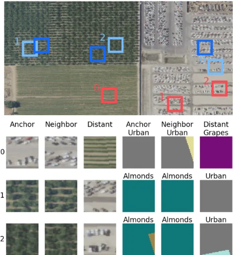
Figure 1: Top: Light blue boxes denote anchor tiles, dark blue neighbor tiles, and red distant tiles. Bottom: Tile triplets corresponding to the top panel. The columns show anchor, neighbor, and distant tiles and their respective CDL class labels. Anchor and neighbor tiles tend to be the same class, while anchor and distant tend to be different.
embeddings’l2-norms, we constrain the network to gener-ate embeddings within a hypersphere and encourage a better representation, not just a bigger one. Given a dataset ofN
tile triplets, our full training objective is
min
θ N X
i=1
h
L(t(i)) +λ
||za(i)||2+||zn(i)||2+||z(di)||2
i
, (2)
where λ controls the regularization strength and za(i) =
fθ(t
(i)
a )∈Rdand similarly forz(ni)andz
(i)
d .
2.3
Triplet sampling
The sampling procedure for ta,tn, andtd is described by
two parameters:
• Tile sizedefines the pixel width and height of a single tile.
• Neighborhooddefines the region around the anchor tile from which to sample the neighbor tile. In our implemen-tation, if the neighborhood is 100 pixels, then the center of the neighbor tile must be within 100 pixels of the anchor tile center both vertically and horizontally. The distant tile is sampled at random from outside this region.
Algorithm 1SampleTileTriplets(D, N, s, r)
1: Input:Image dataset D, number of tripletsN, tile size s,
neighborhood radiusr
2: Output:Tile tripletsT ={(t(ai), t (i) n , t
(i) d )}
N i=1 3:
4: Initialize tile tripletsT ={} 5: fori←1, Ndo
6: t(ai)←SAMPLETILE(D, s)
7: t(ni)←SAMPLETILE(NEIGHBORHOOD(D, r, t (i) a ), s) 8: t(di)←SAMPLETILE(¬NEIGHBORHOOD(D, r, t(ai)), s) 9: UpdateT ←T∪(ta(i), t(ni), t(di))
10: end for 11: returnT 12:
13: functionSAMPLETILE(A, s)
14: t←Sample tile of sizesuniformly at random fromA 15: returnt
16: end function 17:
18: functionNEIGHBORHOOD(D, r, t)
19: A←Subset ofDwithin radiusrof tilet 20: returnA
21: end function
enough to capture intra-class (and potentially some inter-class) variability. In practice, we find that plotting some ex-ample triplets as in Fig. 1 allowed us to find reasonable val-ues for these parameters. Results across tile size and neigh-borhood on our land cover classification experiment are re-ported in Table A3.1
Pseudocode for sampling a dataset of triplets is given in Algorithm 1. Note that no knowledge of actual geographi-cal locations is needed, so Tile2Vec can be applied to any dataset without knowledge of the data collection procedure.
2.4
Scalability
Like most deep learning algorithms, the Tile2Vec objec-tive (Eq. 2) allows for mini-batch training on large datasets. More importantly, the use of the triplet loss allows the train-ing dataset to grow with aquadraticrelationship relative to the size of the available remote sensing data. Concretely, assume that for a given remote sensing dataset we have a sampling budget ofN triplets. If we train using the straight-forward approach of Eq. 2, we will iterate overN training examples in each epoch. However, we notice that in most cases the area covered by our dataset is much larger than the area of a single neighborhood. For any tilet, the likeli-hood that any particulart0in the other(N−1)tiles is in its neighborhood is extremely low. Therefore, at training time we can match any(ta, tn)pair with any of the3N tiles in
the dataset to increase the number of unique example triplets that the network sees fromO(N)toO(N2).
In practice, we find that combining Tile2Vec with this data augmentation scheme to create massive datasets results in an algorithm that is easy to train, robust to hyperparameter choices, and resistant to overfitting. This point will be revis-ited in section 4.1.
1
Appendix available at https://arxiv.org/abs/1805.02855.
3
Datasets
We evaluate Tile2Vec on several widely-used classes of re-mote sensing imagery, as well as a non-image dataset of country characteristics. A brief overview of data organized by experiment is given here, with more detailed descriptions in Appendix A.5.
3.1
Land cover classification
We first evaluate Tile2Vec on a land use classification task — predicting what is on the Earth’s surface from remotely sensed imagery — that uses the following two datasets: The USDA’sNational Agriculture Imagery Program (NAIP)
provides aerial imagery for public use that has four spectral bands — red (R), green (G), blue (B), and infrared (N) — at 0.6 m ground resolution. We obtain an image of Central Valley, California near the city of Fresno for the year 2016 (Fig. 2), spanning latitudes [36.45,37.05] and longitudes
[−120.25,−119.65]. TheCropland Data Layer (CDL)is a raster geo-referenced land cover map collected by the USDA for the continental United States (USDA-NASS 2016). Of-fered at 30 m resolution, it includes 132 class labels span-ning crops, developed areas, forest, water, and more. In our NAIP dataset, we observe 66 CDL classes (Fig. A10). We use CDL as ground truth for evaluation by upsampling it to NAIP resolution.
3.2
Latent space interpolation and visual analogy
We explore Tile2Vec embeddings by visualizing linearly in-terpolated tiles in the learned feature space and performing visual analogies on two datasets. Tiles sampled fromNAIP
are used in the latent space interpolation evaluation. The USGS and NASA’sLandsat 8 satelliteprovide moderate-resolution (30 m) multispectral imagery on a 16-day col-lection cycle. Landsat datasets are public and widely used in agricultural, environmental, and other scientific applica-tions. We generate median Landsat 8 composites containing 7 spectral bands over the urban and rural areas of three ma-jor US cities — San Francisco, New York City, and Boston — for a visual analogy evaluation.
3.3
Poverty prediction in Uganda
We evaluate the regression task of predicting local poverty levels from Landsat 7 composites of Uganda from 2009-2011 containing 5 spectral bands. The World Bank’sLiving Standards Measurement Study (LSMS)surveys measure annual consumption expenditure at the household and vil-lage levels — these measurements are the basis for deter-mining international standards for extreme poverty. We use the Uganda 2011-12 survey as labels for the poverty predic-tion task described in (Jean et al. 2016).
3.4
Worldwide country health index prediction
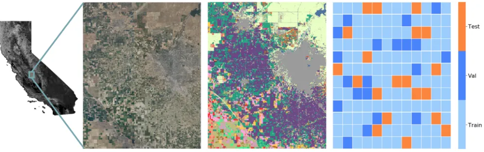
Figure 2:Left:Our NAIP aerial imagery covers 2500 km2around Fresno, California.Center:Land cover types as labeled by the Cropland Data Layer (CDL, see Section 3.1) show a highly heterogeneous landscape; each color represents a different CDL class.Right:For the land cover classification task, we split the dataset spatially into train, validation, and test sets.
compiled by the U.S. Central Intelligence Agency contain-ing information on the governments, economies, energy sys-tems, and societies of 267 world entities (Factbook 2015). We extract a dataset from the 2015 Factbook that contains 73 real-valued features (e.g., infant mortality rate, GDP per capita, crude oil production) for 242 countries.
4
Experiments
4.1
Land cover classification using aerial imagery
We train Tile2Vec embeddings on 100k triplets sampled from the NAIP dataset. The Tile2Vec CNN is a ResNet-18 architecture (He et al. 2016) modified for28×28 CIFAR-10 images (1) with an additional residual block to handle our larger input and (2) without the final classification layer. Each of the 300k50×50NAIP tiles is labeled with the mode CDL land cover class and our evaluation metric is classifi-cation accuracy on this label.
To ensure that training and test sets are spatially disjoint, we split the area into a12×12grid of rectangular blocks, which we then partitioned randomly into train (104 blocks), validation (20 blocks), and test (20 blocks) (Fig. 2, right). Each of these blocks is just over 17 km2 in size, roughly 5000 times the size of each tile. By splitting the dataset at the block level, we are able to reduce the spatial autocorrelation and estimate generalization error with minimal inflation.
Tile2Vec hyperparameter optimization We tune the two main hyperparameters of Algorithm 1 by searching over a grid of tile sizes and neighborhoods. We run the CDL land cover classification experiment 20 times in total, us-ing combinations of tile size in[25,50,75,100]and neigh-borhood radius in [50,100,500,1000,None], where None indicates that both the neighbor and distant tiles are sam-pled from anywhere in the dataset (i.e., infinite radius). The resulting accuracies are reported in Table A1. Results sug-gest that on this task and dataset, a neighborhood radius of 100 pixels strikes the ideal balance between sampling se-mantically similar tiles and capturing intra-class variabil-ity, though classification accuracy remains higher than the
model with infinite radius even when the neighborhood is increased to 1000 pixels. Accuracy also increases with tile size, which can be attributed to greater imbalance of labels at larger tile sizes (Appendix A.4) as well as greater avail-able spatial context for classification.
Because CDL labels are at a resolution (30 m) equivalent to 50 NAIP pixels (0.6 m), we ultimately choose a tile size of 50 and neighborhood of 100 pixels for the land cover classi-fication task. For consistency, subsequent experiments also use these default hyperparameters. Although these default hyperparameters yield high performance in most cases, they should generally be optimized for new datasets and tasks.
Unsupervised learning baselines We compare Tile2Vec to a number of unsupervised feature extraction methods. We describe each baseline here, and provide additional training details in Appendix A.1.
• Autoencoder: A convolutional autoencoder is trained on all 300k multispectral tiles, split 90% training and 10% validation. We train until the validation reconstruction er-ror flattens; the encoder is then used to embed tiles into the feature space. The autoencoder achieves good recon-structions on the held-out test set (examples in Appendix A.1).
• Pre-trained ResNet-18: A modified ResNet-18 was trained on resized CIFAR-10 images and used as a fea-ture extractor. Since CIFAR-10 only has RGB channels, this approach only allows for use of the RGB bands of NAIP and illustrates the limitations of transferring mod-els from natural images to remote sensing datasets.
• PCA/ICA: Each RGBN tile of shape (50,50,4) is un-raveled into a vector of length 10,000 and then PCA/ICA is used to compute the first 10 principal components for each tile.
n= 1000 n= 10000
Unsupervised features RF LR MLP RF LR MLP
Tile2Vec 52.6±1.1 53.7±1.3 55.1±1.2 56.9±0.3 59.7±0.3 58.4±0.3
Autoencoder 49.1±0.7 44.7±1.0 52.0±1.0 53.1±0.2 55.6±0.2 57.2±0.4 Pre-trained ResNet-18 47.7±0.6 48.4±0.8 49.9±1.7 50.6±0.2 53.7±0.2 54.4±0.4 PCA 46.9±0.8 50.2±0.4 43.6±5.3 50.1±0.3 51.1±0.1 52.4±0.3 ICA 47.7±0.6 50.1±0.6 46.7±3.1 50.4±0.4 51.1±0.1 52.5±0.2 K-Means 43.1±0.8 49.4±0.4 44.5±3.9 45.6±0.5 50.0±0.1 50.5±0.2
Table 1: Comparison of Tile2Vec features to unsupervised baselines on the CDL classification task in Section 4.1. Random forest (RF), logistic regression (LR), and multilayer perceptron (MLP) classifiers are trained over 10 trials ofn= 1000and
n= 10000randomly sampled labels, with mean accuracies and standard deviations reported.
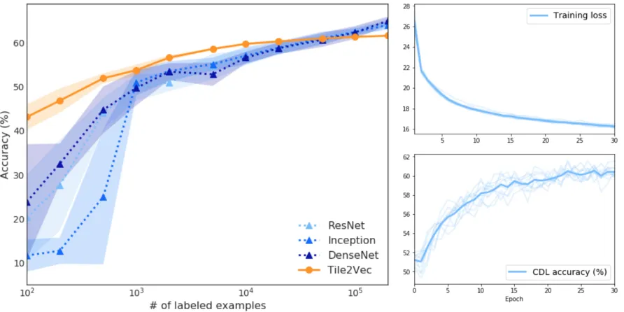
Figure 3:Left:Logistic regression on Tile2Vec unsupervised features outperforms supervised CNNs until 50k labeled exam-ples.Right:The Tile2Vec triplet loss decreases steadily and downstream classification accuracy tracks the loss.
As shown in Table 1, the features learned by Tile2Vec out-perform other unsupervised features when used by random forest (RF), logistic regression (LR), and multilayer percep-tron (MLP) classifiers trained onn = 1000orn = 10000
labels. We also trained a DCGAN (Radford, Metz, and Chin-tala 2015) as a generative modeling approach to unsuper-vised feature learning. Although we were able to gener-ate reasonable samples, features learned by the discrimina-tor performed poorly — samples and results can be found in Appendix A.1. Approaches based on variational autoen-coders (VAEs) would also provide intriguing baselines, but we are unaware of existing models capable of capturing complex multispectral image distributions.
Supervised learning comparisons Surprisingly, our Tile2Vec features are also able to outperform fully-supervised CNNs trained directly on the classification task with large amounts of labeled data. Fig. 3 shows that ap-plying logistic regression on Tile2Vec features beats several state-of-the-art supervised architectures (He et al. 2016;
Szegedy et al. 2015; Huang et al. 2017) trained on as many as 50k CDL labels. We emphasize that the Tile2Vec CNN and the supervised ResNet share the same architecture, so logistic regression in Fig. 3 is directly comparable to the classification layers of the supervised architectures. Similar results for random forest and multilayer perceptron classifiers can be found in Appendix A.4.
Latent space interpolation We further explore the learned representations with a latent space interpolation ex-periment shown in Fig. 4. Here, we start with the Tile2Vec embeddings of a field tile and an urban tile and linearly in-terpolate between the two. At each point along the interpo-lation, we search for the five nearest neighbors in the la-tent space and display the corresponding tiles. As we move through the semantically meaningful latent space, we re-cover tiles that are more and more developed.
Figure 4:Left:Linear interpolation in the latent space at equal intervals between representations of rural and urban images. Below, we show 5 nearest neighbors in the latent space to each interpolated vector.Right:Starting with a rural NYC embedding, we add urban SF and subtract rural SF to successfully discover urban NYC tiles. More visual analogies are shown in Fig. A6.
ranging from 0.1 to 100 and found little effect on accuracy. Using a margin of 50, we trained Tile2Vec for 10 trials with different random initializations and show the results in Fig. 3. The training loss is stable from epoch to epoch, consis-tently decreasing, and most importantly, a good proxy for unsupervised feature quality as measured by performance on the downstream task (Fig. 3, bottom right). By combining explicit regularization (Eq. 2) with the data augmentation scheme described in Section 2.4, we observe that Tile2Vec does not seem to overfit even when trained for many epochs.
4.2
Visual analogies across US cities
To evaluate Tile2Vec qualitatively, we explore three major metropolitan areas of the United States: San Francisco, New York City, and Boston. First, we train a Tile2Vec model on the San Francisco dataset only. Then we use the trained model to embed tiles from all three cities. As shown in Fig. 4 and A6, these learned representations allow us to perform arithmetic in the latent space, orvisual analogies(Radford, Metz, and Chintala 2015). By adding and subtracting vec-tors in the latent space, we can recover image tiles that are semantically expected given the operations applied.
Here we use Landsat images with 7 spectral bands, demonstrating that Tile2Vec can be applied effectively to highly multispectral datasets. Tile2Vec can also learn rep-resentations at multiple scales: each Landsat 8 (30 m resolu-tion) tile covers 2.25 km2, while the NAIP and DigitalGlobe
tiles are 2500 times smaller. Finally, Tile2Vec learns robust representations that allow for domain adaptation or transfer learning, as the three datasets have widely varying spectral distributions (Fig. A9).
4.3
Poverty prediction from satellite imagery
Next, we apply Tile2Vec to predict annual consumption ex-penditures in Uganda from satellite imagery. Accurate mea-surements of poverty are essential for both research and pol-icy, but reliable data is limited in the developing world — machine learning methods that are still effective when la-beled data is scarce could help to fill these critical gaps.
Features d kNN RF RR
Tile2Vec 10 77.5±1.0 76.0±1.3 69.6±1.0
Non-health 60 62.8±1.5 72.1±1.6 68.7±1.7 Locations 2 69.3±1.0 67.7±2.6 11.6±1.5
Table 2: Predicting health index using Tile2Vec features ver-sus non-health features and locations (i.e.,{lat, lon}). Here,
dis feature dimension, kNN is k-nearest neighbors, RF is random forest, and RR is ridge regression. Hyperparameters (e.g.,kand regularization strength) are tuned for each fea-ture set. We report averager2and standard deviation for 10
trials of 3-fold cross-validation.
The previous state-of-the-art result used a transfer learn-ing approach in which a CNN is trained to predict night-time lights (a proxy for poverty) from daynight-time satellite im-ages — the features from this model are then used to pre-dict consumption expenditures (Jean et al. 2016). We use the same LSMS survey preprocessing pipeline and ridge re-gression evaluation (see Appendix A.2). Evaluating over10
trials of 5-fold cross-validation, we report an averager2 of
0.496±0.014compared tor2= 0.41for the transfer learn-ing approach — this is achieved with publicly available agery with much lower resolution than the proprietary im-ages used in (Jean et al. 2016) (30 m vs. 2.4 m).
4.4
Generalizing to other spatial data: Predicting
country health indices
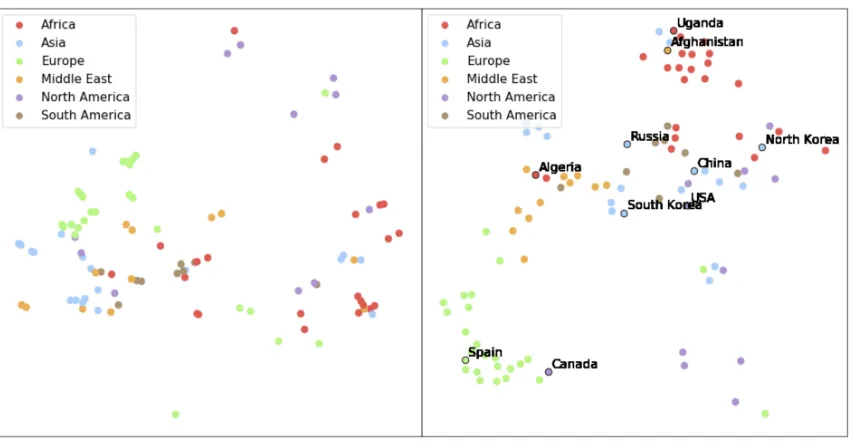
Figure 5:Left:The 60 non-health country features visualized using t-SNE. Spatial relationships are preserved for some clusters, but not for others.Right:The 10-dimensional Tile2Vec embeddings visualized using t-SNE. The latent space now respects both spatial and characteristic similarities. Several countries are annotated to highlight interesting relationships: North Korea and South Korea are embedded far apart even though they are spatial neighbors; USA, South Korea, and China are embedded close together though they are geographically separated.
As shown in Table 2, the embeddings learned by Tile2Vec on this small spatial dataset (N = 242) outperform both the original features and approaches that explicitly use spatial information. Fig. 5 shows the original 60-dimensional fea-ture vectors as well as the 10-dimensional learned Tile2Vec embeddings projected down to two dimensions using t-SNE (van der Maaten and Hinton 2008). While there is some ge-ographic grouping of countries in projecting down the orig-inal features, the Tile2Vec embeddings appear to capture both geographic proximity and socioeconomic similarity.
In this experiment, the Haversine formula was used to compute the great-circle distance between pairs of countries in kilometers — future work could explore using distance functions more meaningful to the application at hand, e.g., shared borders or trade volume.
5
Related Work
Our inspiration for using spatial context to learn repre-sentations originated from continuous word reprerepre-sentations like Word2vec and GloVe (Mikolov et al. 2013b; 2013a; Pennington, Socher, and Manning 2014). In NLP, the distri-butional hypothesis can be summarized as “a word is char-acterized by the company it keeps” — words that appear in the same context likely have similar semantics. We apply this concept to remote sensing data, with multispectral im-age tiles as the atomic unit analogous to individual words in NLP, and geospatial neighborhoods as the “company” that these tiles keep. A related, supervised version of this idea is the patch2vec algorithm (Fried, Avidan, and Cohen-Or 2017), which its authors describe as learning “globally con-sistent image patch representations”. Working with natural
images, they use a very similar triplet loss (first introduced in (Hoffer and Ailon 2015)), but sample their patches with su-pervision from an annotated semantic segmentation dataset. Unsupervised learning for visual data is an active area of research and thus impossible to summarize concisely, but we attempt a brief overview of the most relevant topics here. The three main classes of deep generative models — likelihood-based variational autoencoders (VAEs) (Kingma and Welling 2013), likelihood-free generative adversarial networks (GANs) (Goodfellow et al. 2014), and various au-toregressive models (Oord, Kalchbrenner, and Kavukcuoglu 2016; van den Oord et al. 2016) — attempt to learn the generating data distribution from training samples. Other re-lated lines of work use spatial or temporal context to learn high-level image representations. Some strategies for using spatial context involve predicting the relative positions of patches sampled from within an image (Noroozi and Favaro 2016; Doersch, Gupta, and Efros 2015) or trying to fill in missing portions of an image (in-painting) (Pathak et al. 2016). In videos, nearby frames can be used to learn tem-poral embeddings (Ramanathan et al. 2015); other methods leveraging the temporal coherence and invariances of videos for feature learning have also been proposed (Misra, Zitnick, and Hebert 2016; Wang and Gupta 2015).
6
Conclusion
and collected via aerial or satellite sensors, and even to non-image datasets. Tile2Vec outperforms other unsuper-vised feature extraction techniques on a difficult classifi-cation task — surprisingly, it even outperforms supervised CNNs trained on 50k labeled examples.
In this paper, we focus on exploitingspatialcoherence, but many geospatial datasets also include sequences of data collected over time. Temporal patterns can be highly infor-mative (e.g., seasonality, crop cycles), and we plan to ex-plore this aspect in future work. Remote sensing data have largely been unexplored by the machine learning commu-nity — more research in these areas could result in enormous progress on many problems of global significance.
Acknowledgements
This research was supported by NSF (#1651565, #1522054, #1733686), ONR, Sony, and FLI. NJ was supported by the Department of Defense (DoD) through the National Defense Science & Engineering Graduate Fellowship (NDSEG) Pro-gram.
References
Doersch, C.; Gupta, A.; and Efros, A. A. 2015. Unsupervised vi-sual representation learning by context prediction. InProceedings
of the IEEE International Conference on Computer Vision, 1422–
1430.
Factbook, C. 2015. The World Factbook; 2010. http://www.cia. gov/library/publications/the-world-factbook. Accessed: 2018-01-20.
Foody, G. M. 2003. Remote sensing of tropical forest environ-ments: Towards the monitoring of environmental resources for sus-tainable development. International Journal of Remote Sensing
24(20):4035–4046.
Fried, O.; Avidan, S.; and Cohen-Or, D. 2017. Patch2Vec: Glob-ally consistent image patch representation. InComputer Graphics
Forum, volume 36, 183–194. Wiley Online Library.
Goodfellow, I.; Pouget-Abadie, J.; Mirza, M.; Xu, B.; Warde-Farley, D.; Ozair, S.; Courville, A.; and Bengio, Y. 2014. Gen-erative adversarial nets. InAdvances in Neural Information
Pro-cessing Systems, 2672–2680.
He, K.; Zhang, X.; Ren, S.; and Sun, J. 2016. Deep residual learn-ing for image recognition. InProceedings of the IEEE conference
on Computer Vision and Pattern Recognition, 770–778.
Hoffer, E., and Ailon, N. 2015. Deep metric learning using triplet network. InInternational Workshop on Similarity-Based Pattern
Recognition, 84–92. Springer.
Huang, G.; Liu, Z.; Weinberger, K. Q.; and van der Maaten, L. 2017. Densely connected convolutional networks. InProceedings of the IEEE conference on Computer Vision and Pattern Recogni-tion, volume 1, 3.
Jean, N.; Burke, M.; Xie, M.; Davis, W. M.; Lobell, D. B.; and Er-mon, S. 2016. Combining satellite imagery and machine learning to predict poverty.Science353(6301):790–794.
Kingma, D. P., and Welling, M. 2013. Auto-encoding variational bayes.arXiv preprint arXiv:1312.6114.
Krizhevsky, A.; Sutskever, I.; and Hinton, G. 2012. ImageNet clas-sification with deep convolutional neural networks. InAdvances in
Neural Information Processing Systems, 1097–1105.
Levy, O., and Goldberg, Y. 2014. Neural word embedding as im-plicit matrix factorization. InAdvances in Neural Information
Pro-cessing Systems, 2177–2185.
Mikolov, T.; Chen, K.; Corrado, G.; and Dean, J. 2013a. Efficient estimation of word representations in vector space. arXiv preprint
arXiv:1301.3781.
Mikolov, T.; Sutskever, I.; Chen, K.; Corrado, G. S.; and Dean, J. 2013b. Distributed representations of words and phrases and their compositionality. InAdvances in Neural Information Processing
Systems, 3111–3119.
Misra, I.; Zitnick, C. L.; and Hebert, M. 2016. Shuffle and learn: unsupervised learning using temporal order verification. In
Euro-pean Conference on Computer Vision, 527–544. Springer.
Mulla, D. J. 2013. Twenty five years of remote sensing in pre-cision agriculture: Key advances and remaining knowledge gaps.
Biosystems Engineering114(4):358 – 371. Special Issue: Sensing
Technologies for Sustainable Agriculture.
Noroozi, M., and Favaro, P. 2016. Unsupervised learning of visual representations by solving jigsaw puzzles. InEuropean Conference
on Computer Vision, 69–84. Springer.
Oord, A. v. d.; Kalchbrenner, N.; and Kavukcuoglu, K. 2016. Pixel recurrent neural networks.arXiv preprint arXiv:1601.06759. Oshri, B.; Hu, A.; Adelson, P.; Chen, X.; Dupas, P.; Weinstein, J.; Burke, M.; Lobell, D.; and Ermon, S. 2018. Infrastructure qual-ity assessment in africa using satellite imagery and deep learning.
Proc. 24th ACM SIGKDD Conference.
Pathak, D.; Krahenbuhl, P.; Donahue, J.; Darrell, T.; and Efros, A. A. 2016. Context encoders: Feature learning by inpainting.
InProceedings of the IEEE Conference on Computer Vision and
Pattern Recognition, 2536–2544.
Pennington, J.; Socher, R.; and Manning, C. 2014. Glove: Global vectors for word representation. InProceedings of the 2014 Con-ference on Empirical Methods in Natural Language Processing
(EMNLP), 1532–1543.
Radford, A.; Metz, L.; and Chintala, S. 2015. Unsupervised rep-resentation learning with deep convolutional generative adversarial networks.arXiv preprint arXiv:1511.06434.
Ramanathan, V.; Tang, K.; Mori, G.; and Fei-Fei, L. 2015. Learn-ing temporal embeddLearn-ings for complex video analysis. In
Proceed-ings of the IEEE International Conference on Computer Vision,
4471–4479.
Szegedy, C.; Liu, W.; Jia, Y.; Sermanet, P.; Reed, S.; Anguelov, D.; Erhan, D.; Vanhoucke, V.; Rabinovich, A.; et al. 2015. Going deeper with convolutions. InProceedings of the IEEE Conference
on Computer Vision and Pattern Recognition.
USDA-NASS. 2016. USDA National Agricultural Statistics Ser-vice Cropland Data Layer. published crop-specific data layer [on-line].
van den Oord, A.; Kalchbrenner, N.; Espeholt, L.; Vinyals, O.; Graves, A.; et al. 2016. Conditional image generation with pix-elcnn decoders. In Advances in Neural Information Processing
Systems, 4790–4798.
van der Maaten, L., and Hinton, G. 2008. Visualizing high-dimensional data using t-SNE. Journal of Machine Learning
Re-search9:2579–2605.
Wang, X., and Gupta, A. 2015. Unsupervised learning of visual representations using videos.arXiv preprint arXiv:1505.00687. Xie, M.; Jean, N.; Burke, M.; Lobell, D.; and Ermon, S. 2016. Transfer learning from deep features for remote sensing and poverty mapping. InProceedings of the Thirtieth AAAI Conference