The Thirty-Third AAAI Conference on Artificial Intelligence (AAAI-19)
Partial Multi-Label Learning via Credible Label Elicitation
Jun-Peng Fang,
1,2Min-Ling Zhang
1,2,3,∗1School of Computer Science and Engineering, Southeast University, Nanjing 210096, China
2Key Laboratory of Computer Network and Information Integration (Southeast University), Ministry of Education, China 3Collaborative Innovation Center of Wireless Communications Technology, China
[email protected], [email protected]* (corresponding author)
Abstract
In partial multi-label learning (PML), each training example is associated with multiple candidate labels which are only partially valid. The task of PML naturally arises in learning scenarios with inaccurate supervision, and the goal is to in-duce a multi-label predictor which can assign a set of proper labels for unseen instance. To learn from PML training exam-ples, the training procedure is prone to be misled by the false positive labels concealed in candidate label set. In light of this major difficulty, a novel two-stage PML approach is proposed which works by eliciting credible labels from the candidate label set for model induction. In this way, most false positive labels are expected to be excluded from the training proce-dure. Specifically, in the first stage, the labeling confidence of candidate label for each PML training example is estimated via iterative label propagation. In the second stage, by utiliz-ing credible labels with high labelutiliz-ing confidence, multi-label predictor is induced via pairwise label ranking with virtual la-bel splitting or maximum a posteriori (MAP) reasoning. Ex-tensive experiments on synthetic as well as real-world data sets clearly validate the effectiveness of credible label elicita-tion in learning from PML examples.
Introduction
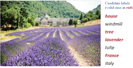
Partial multi-label learning deals with one particular learn-ing framework with inaccurate supervision, where multiple candidate labels are assigned to each training example which are only partially valid. The need to learn from PML ex-amples naturally arises in many real-world scenarios, where accurate supervision information is difficult to be obtained from the collected data (Zhou 2018; Xie and Huang 2018). For instance, in crowdsourcing image tagging (Figure 1), among the set of candidate labels given by crowdsourcing annotators only some of them are valid ones due to potential unreliable annotators. The task of partial multi-label learn-ing is to learn a multi-label predictor from PML trainlearn-ing ex-amples which can assign a set of proper labels for the unseen instance.
Formally, letX = Rd denote thed-dimensional feature
space and Y = {y1, y2, . . . , yq} denote the output space
withq possible class labels. Furthermore, given the PML training setD= {(xi, Yi) | 1 ≤i ≤ m}, wherexi ∈ X
Copyright c2019, Association for the Advancement of Artificial Intelligence (www.aaai.org). All rights reserved.
Figure 1: An examplar partial multi-label learning scenario. In crowdsourcing image tagging, among the set of 7 can-didate labels given by crowdscourcing annotators, only 4 of them are valid ones includinghouse,tree,lavenderand
France.
is a d-dimensional feature vector andYi ⊆ Y is the set of
candidate labels associated withxi. The key assumption of
partial multi-label learning lies in that the ground-truth la-bels Yei ⊆ Y for xi reside in the candidate label set, i.e.
e
Yi ⊆ Yi, and are not directly accessible to the learning
al-gorithm. Accordingly, the task of PML is to induce a multi-label predictorf :X 7→2YfromD.
A straightforward strategy to learn from PML examples is to treat all the candidate labels inYias ground-truth ones,
and then apply off-the-shelf multi-label learning algorithms (Zhang and Zhou 2014; Gibaja and Ventura 2015) to induce the desired multi-label predictor. Obviously, the resulting multi-label training procedure will be significantly affected by the labeling noise brought by false positive labels inYi.
One recent attempt towards PML works by utilizing the con-fidence of each candidate label being the ground-truth one (Xie and Huang 2018), where confidence scores and predic-tive model are optimized in an alternapredic-tive manner by mini-mizing the confidence-weighted ranking loss between can-didate and non-cancan-didate labels. Nonetheless, the estimated confidence scores would be error-prone especially when the proportion of false positive labels is high, which in turn will impact the predictive model due to the alternative optimiza-tion procedure.
are concealed in the candidate label set of PML training ex-amples, a novel approach named PARTICLE, i.e. PARTIal multi-label learning via Credible Label Elicitation, is pro-posed in this paper. The basic idea of PARTICLE is to mit-igate the negative impact of false positive labels by elicit-ing credible labels from candidate label set, which will be treated as reliable labeling information for subsequent model induction. Briefly, in the first stage, credible labels with high labeling confidence are identified via iterative label propa-gation. In the second stage, by making use of the identified credible labels, multi-label predictor is induced via pairwise label ranking with virtual label splitting or maximum a pos-teriori reasoning. Comprehensive experimental studies show that credible label elicitation serves as an effective strategy to solve the partial multi-label learning problem.
The rest of this paper is organized as follows. Firstly, re-lated works on partial multi-label learning are briefly dis-cussed. Secondly, technical details of the proposed PARTI
-CLEapproach are presented. Thirdly, detailed experimental results are reported. Finally, we conclude this paper.
Related Work
Partial multi-label learning is closely related to two popular learning frameworks, namely multi-label learning (Zhang and Zhou 2014; Gibaja and Ventura 2015; Zhou and Zhang 2017) and partial label learning (Cour, Sapp, and Taskar 2011; Liu and Dietterich 2012; Zhang, Yu, and Tang 2017). In multi-label learning (MLL), each example is associated with multiple valid labels simultaneously. Based on the or-der of correlations being exploited for model training, exist-ing MLL approaches can be roughly categorized into three groups includingfirst-order approaches(Boutell et al. 2004; Zhang et al. 2018), second-order approaches (F¨urnkranz et al. 2008; Li, Song, and Luo 2017), and high-order ap-proaches(Read et al. 2011; Tsoumakas, Katakis, and Vla-havas 2011; Burkhardt and Kramer 2018). Both MLL and PML aim to induce the predictive model which can as-sign proper label set for unseen instance. Nonetheless, the task of PML is more challenging than MLL as the ground-truth labeling information is not directly accessible to PML learning algorithm. There are also studies on weak label learning (Sun, Zhang, and Zhou 2010; Tan et al. 2018; Wei et al. 2018) which considers the case of missing ground-truth labels w.r.t. the associated label set. Weak label learn-ing and PML can be viewed as dual variants of MLL with noisy labeling, where weak label learning assumes false neg-ative labels within irrelevant label set while PML assumes false negative labels within candidate label set.
In partial label learning (PLL), each example is associ-ated with multiple candidate labels among which only one is valid. The task of partial label learning is to induce a multi-class predictive model which can assign one proper label for unseen instance, where existing PLL approaches work by disambiguating the candidate label set (Cour, Sapp, and Taskar 2011; Liu and Dietterich 2012; Yu and Zhang 2017; Gong et al. 2018; Chen, Patel, and Chellappa 2018) or trans-forming partial label learning problem into canonical super-vised learning problems (Chen et al. 2014; Zhang, Yu, and Tang 2017; Wu and Zhang 2018). Both PLL and PML learn
from training examples with labeling noise where false pos-itive labels reside in the candidate label set. Nonetheless, the task of PML is more challenging than PLL as a multi-label predictor rather than single-label predictor needs to be in-duced from PML training examples.
To solve the partial multi-label learning problem, one most straightforward strategy is to treat all candidate labels as ground-truth ones. In this way, any off-the-shelf multi-label learning algorithms can be applied to induce the de-sired multi-label predictor. Nevertheless, it is obvious that this straightforward strategy tends to suffer from the false positive labels concealed in candidate label set. Another re-cent strategy (Xie and Huang 2018) learns from PML exam-ples by estimating the ground-truth labeling confidence of each candidate label, where the estimated confidence scores are incorporated into an alternative optimization procedure for model induction. Due to the alternative nature of opti-mization, estimation errors on confidence scores will keep impairing the coupled predictive model, especially when the proportion of false positive labels is high.
In the next section, a two-stage partial multi-label learn-ing strategy based on credible label elicitation will be intro-duced, which aims to mitigate the negative impact of false positive labels by focusing on reliable labeling information.
The P
ARTICLEApproach
Credible Label Elicitation
In the first stage, PARTICLEelicits credible labels from the candidate label set via an iterative label propagation proce-dure. Given the PML training setD={(xi, Yi)| 1≤i≤
m}, a weighted directed graphG = (V, E,W)is instan-tiated based onkNN minimum error reconstruction. Here, V ={xi | 1 ≤i ≤m}corresponds to the set of training
instances andE = {(xi,xj)| i ∈ N(xj),1 ≤ j ≤m} withN(xj)being the index set ofxj’sknearest neighbors
inD.
For the weight matrix W = [w1,w2, . . . ,wm]>, the weight vectorwj = [w1,j, w2,j, . . . , wm,j]>(1 ≤j ≤m)
is optimized by solving the following minimum error recon-struction problem:
minwj xj−
Xm
i=1wi,j·xi 2
2 (1)
s.t. wi,j≥0 (i∈ N(xj))
wi,j= 0 (i /∈ N(xj))
Conceptually, the goal of Eq.(1) is to minimize the loss of reconstructing xj from its k nearest neighbors with non-negative weights. Accordingly, the solution to the linear least square problem of Eq.(1) can be obtained by applying off-the-shelf quadratic programming (QP) solver.
LetH=WD−1be the propagation matrix by normaliz-ing the columns ofW, whereD= diag [d1, d2, . . . , dm]is
the diagonal matrix withdj =P m
i=1wi,j. Furthermore, let
F= [fi,c]m×qbe anm×qmatrix with non-negative entries
wherefi,c≥0is assumed to represent the confidence ofyc
the initial labeling confidence matrixF(0)is configured as:
∀1≤i≤m: fi,c(0)=
( 1
|Yi|, if yc∈Yi
0, otherwise (2)
Therefore, the initial labeling confidence is evenly dis-tributed over the candidate label set. For thet-th iteration,F is updated by propagating current labeling confidence over H:
b
F(t)=α·H>F(t−1)+ (1−α)·F(0) (3) Here, the parameterα ∈ [0,1]controls the labeling infor-mation inherited from iterative propagation and the initial labeling confidenceF(0). After that,Fb(t)will be re-scaled
intoF(t)by normalizing each row w.r.t. the candidate label set:
∀1≤i≤m: fi,c(t)=
ˆ
fi,c(t) P
yl∈Yifˆ (t) i,l
, if yc∈Yi
0, otherwise
(4)
LetF∗denote the final labeling confidence matrix when the
iterative label propagation procedure terminates1, it is fea-sible to elicit credible labels for each PML training exam-ple by identifying candidate labels with high labeling confi-dence w.r.tF∗.
Nonetheless, to reduce the risk of overfitting with label propagation, PARTICLE fulfills the elicitation task by fur-ther performingkNN aggregation. Forxj and itsknearest neighbors in N(xj), the aggregation weight vectorωj = [ω1j, ω2j, . . . , ωjm]>is set as:
∀1≤i≤m:
wji =
(
1− dist(xi,xj)
P
xk∈N(xj)dist(xk,xj), if xi∈ N(xj)
0, otherwise
(5)
Here, dist(xi,xj) calculates the Euclidean distance be-tweenxjand its neighboring examplexi. Then, the result-ing labelresult-ing confidence vector λj = [λj
1, λ
j
2, . . . , λjq]> for xjis obtained by aggregatingF∗withωj:
λj = F∗>·ωj (6)
Thereafter, the credible label setYjCforxjis determined by thresholdingλj:2
YjC =
{yl|λjl ≥thr, yl∈Yj} [
{yl∗|yl∗= argmax
yl∈Yj
λjl} (7)
In other words,YjC ⊆Yjis formed by credible labels whose
labeling confidence are greater than the thresholding param-eterthr ∈[0,1]. The one with highest labeling confidence (i.e.yl∗) also belongs toYjCso as to avoid the potential case of empty credible label set.
1The iterative label propagation procedure terminates when
F(t)does not change or the maximum number of iterations (1,000 in this paper) is reached.
2To facilitate the thresholding operation,λjis further
normal-ized to [0,1] withλjl = λ
j
l−min1≤l≤qλjl
max1≤l≤qλjl−min1≤l≤qλjl .
Table 1: The pseudo-code of PARTICLE.
Inputs:
D: PML training set{(xi, Yi)|1≤i≤m}
(xi∈ X, Yi⊆ Y,X=Rd,Y={y1, y2, . . . , yq}) k: number of nearest neighbors considered
α: balancing parameter thr: thresholding parameter B: binary training algorithm
mode: virtual label splittingorMAP reasoning x: unseen instance
Outputs:
Y: predicted label set forx
Process:
1: Instantiate the weighted graphG= (V, E,W)by solv-ing Eq.(1) withkNN minimum error reconstruction;
2: InitializeF(0) according to Eq.(2) and obtain the final labeling confidence matrixF∗ by conducting iterative label propagation according to Eq.(3) and Eq.(4);
3: Identify the credible label set YjC for each example
xj (1 ≤ j ≤ m) according to Eq.(7) (together with
Eq.(5) and Eq.(6));
4: For each label pair(yu, yz) (1≤u < z≤q), generate
binary training setDC
uzaccording to Eq.(8); 5: Induce binary classifierguz←[B(D
C uz); 6: switchmodedo
7: casevirtual label splitting
8: For each labelyu(1≤u≤q), generate binary
training setDC
uV according to Eq.(9); 9: Induce binary classifierguV ←[B(D
C uV); 10: ReturnY =f(x)according to Eq.(12) (together
with Eq.(10) and Eq.(11));
11: caseMAP reasoning
12: For each labelyu(1≤u≤q), set the counting
statisticCuaccording to Eq.(13);
13: ReturnY =f(x)according to Eq.(14) (together with Eqs.(15)-(18));
14: end switch
Predictive Model Induction
In the second stage, PARTICLE aims to induce the multi-label predictive model by utilizing credible multi-labels elicited in the first stage.
Specifically, letDC ={(xi, YC
i ) | 1 ≤ i ≤ m}denote
the transformed PML training set where each training exam-plexiis associated with the credible label setYiCother than the original candidate label set Yi. Pairwise label ranking
is tailored to learn from the transformed PML training ex-amples with virtual label splitting or maximum a posteriori (MAP) reasoning, where similar techniques have been suc-cessfully applied to learn from multi-label data (Zhang and Zhou 2007; F¨urnkranz et al. 2008; Zhang and Zhou 2014; Gibaja and Ventura 2015).
The basic idea of pairwise label ranking is to transform the original learning problem into a number of pairwise comparison problems, one for each label pair(yu, yz) (1≤
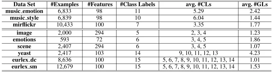
Table 2: Characteristics of the PML experimental data sets. For each PML data set, the average number of candidate labels (avg. #CLs) and the average number of ground-truth labels (avg. #GLs) are also recorded.
Data Set #Examples #Features #Class Labels avg. #CLs avg. #GLs
music emotion 6,833 98 11 5.29 2.42
music style 6,839 98 10 6.04 1.44
mirflickr 10,433 100 7 3.35 1.77
image 2,000 294 5 2, 3, 4 1.23
emotions 593 72 6 3, 4, 5 1.86
scene 2,407 294 6 3, 4, 5 1.07
yeast 2,417 103 14 9, 10, 11, 12, 13 4.23
eurlex dc 8,636 100 15 5, 6, 7, 8, 9, 10, 11, 12, 13, 14 1.01
eurlex sm 12,679 100 15 5, 6, 7, 8, 9, 10, 11, 12, 13, 14 1.53
(xi, YiC)withYiC ⊆Yi, letY¯i=Y \Yibe the
complemen-tary set of candidate label setYiinY.
For each label pair(yu, yz), one binary training set is
gen-erated fromDCas follows:
DC uz=
(xi, ϕ(YiC,Y¯i, yu, yz))| (8)
τ(YiC,Y¯i, yu, yz) = true,1≤i≤m where
τ(YiC,Y¯i, yu, yz) =
true, if (yu∈YiC)∧(yz∈Y¯i) or
(yu∈Y¯i)∧(yz∈YiC)
false, otherwise
ϕ(YiC,Y¯i, yu, yz) =
+1, if (yu∈YiC)∧(yz∈Y¯i)
−1, if (yu∈Y¯i)∧(yz∈YiC)
In other words,xiwill be regarded as one positive or nega-tive training example whenyuandyzhave different
assign-ment w.r.t.YiC andY¯i. Otherwise,xi will not contribute to
the generation of binary training setDC uz.
Given the binary training algorithmB, a total of q
2
bi-nary classifiersguz:X 7→Rcan be induced fromDCuz, i.e.
guz ←[ B(D C
uz). Conceptually, for unseen instance x, the
binary classifier votes foryu if guz(x) > 0 andyz
other-wise. Thereafter, based on the q2
binary classifiers, PAR -TICLEproceeds to predict the set of proper labels forxvia virtual label splitting or MAP reasoning.
Virtual Label Splitting In this case, one virtual labelyV
is introduced to yield qextra binary training sets, one for each class labelyu (1 ≤ u ≤ q). Here, yV serves as an
artificial splitting point between credible labels and non-candidate labels. For each labelyu, one binary training set is
generated fromDCas follows:
DuVC =
(xi, ψ(YiC,Y¯i, yu))| (9)
ζ(YiC,Y¯i, yu) = true,1≤i≤m where
ζ(YiC,Y¯i, yu) =
true, if yu∈YiC oryu∈Y¯i
false, otherwise
ψ(YiC,Y¯i, yu) =
+1, if yu∈YiC
−1, if yu∈Y¯i
In other words,xiwill be regarded as one positive or
nega-tive training example whenyu belongs toYiC orY¯i.
Other-wise,xiwill not contribute to the generation of binary
train-ing setDC uV.
Accordingly, another set of q binary classifiers guV :
X 7→ R can be induced from DuVC as well, i.e. guV ←[ B(DC
uV). Furthermore, let ruz andruV denote the
empiri-cal accuracy of guz andguV in classifying binary training
examples in DC
uz andDCuV respectively. Then, for unseen
instancex, the overall (weighted) votes yielded by q2+q classifiers on each class labelyu(1≤u≤q)and the virtual
labelyV correspond to:
Γ(x, yu) = Xu−1
l=1 rlu·Jglu(x)≤0K+ (10)
Xq
l=u+1rul·Jgul(x)>0K+ruV ·JguV(x)>0K
Γ(x, yV) =
Xq
l=1rlV ·JglV(x)≤0K (11) Here, JπK returns 1 if predicate π holds and 0 otherwise. Thereafter, the predicted label set forxis determined as:
f(x) ={yu|Γ(x, yu)>Γ(x, yV),1≤u≤q} (12)
MAP Reasoning In this case, a simple counting statistic is utilized to facilitate model prediction. For unseen instance
x, let Cu denote the statistic which counts the number of
binary classifiers which vote foryuonx:
Cu= Xu−1
l=1Jglu(x)≤0K+
Xq
l=u+1Jgul(x)>0K (13) Note that0≤Cu≤q−1as among the q2
binary classifiers generated by pairwise label ranking,q−1of them are related to labelyu.
LetHudenote the event thatyuis a relevant label forx,
andP(Hu | Cu) represents the posteriori probability that
Huholds givenCu. Accordingly,P(¬Hu | Cu)represents
the posteriori probability that Hu does not hold given the
same condition. Thereafter, the predicted label set forxis determined by the MAP rule:
f(x) = (14)
{yu|P(Hu|Cu)>P(¬Hu|Cu),1≤u≤q}
Based on Bayes theorem, we have:
P(Hu|Cu)
P(¬Hu|Cu)
= P(Hu)·P(Cu|Hu)
P(¬Hu)·P(Cu| ¬Hu)
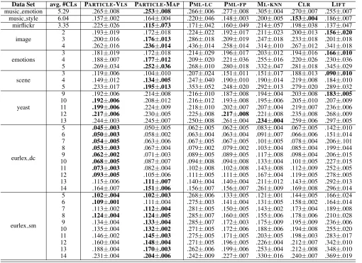
Table 3: Experimental results of each comparing approach in terms ofranking loss, where the best performance (the smaller the better) is shown in bold face.
Data Set avg. #CLs PARTICLE-VLS PARTICLE-MAP PML-LC PML-FP ML-KNN CLR LIFT
music emotion 5.29 .265±.008 .253±.008 .266±.006 .277±.008 .305±.004 .270±.007 .255±.007 music style 6.04 .157±.002 .164±.004 .220±.046 .148±.003 .200±.005 .153±.004 .186±.007 mirflickr 3.35 .225±.026 .115±.073 .171±.042 .160±.049 .214±.057 .198±.038 .137±.047
image
2 .193±.019 .172±.018 .224±.022 .192±.017 .211±.023 .200±.013 .156±.020 3 .200±.016 .176±.013 .286±.018 .209±.019 .247±.018 .233±.018 .201±.018 4 .262±.016 .236±.014 .436±.014 .258±.014 .314±.010 .267±.012 .341±.018
emotions
3 .181±.019 .172±.018 .214±.029 .196±.017 .203±.012 .194±.016 .166±.010 4 .188±.007 .177±.012 .209±.020 .221±.036 .255±.016 .220±.026 .230±.036 5 .269±.034 .252±.036 .268±.010 .280±.018 .332±.047 .281±.018 .345±.029
scene
3 .119±.006 .104±.010 .207±.024 .151±.011 .151±.017 .188±.013 .090±.010 4 .149±.012 .134±.005 .247±.040 .190±.010 .190±.014 .219±.008 .184±.010 5 .233±.017 .195±.013 .353±.052 .248±.020 .292±.013 .279±.020 .289±.032
yeast
9 .192±.006 .214±.008 .216±.010 .187±.008 .194±.004 .203±.008 .183±.005 10 .192±.006 .208±.012 .216±.012 .193±.008 .195±.006 .205±.010 .207±.009 11 .199±.006 .224±.009 .218±.010 .202±.007 .207±.004 .219±.007 .236±.006 12 .217±.006 .230±.005 .225±.008 .217±.008 .221±.008 .235±.008 .268±.009 13 .244±.003 .245±.007 .250±.008 .261±.004 .234±.004 .259±.006 .297±.005
eurlex dc
5 .045±.003 .050±.005 .062±.005 .062±.005 .083±.004 .067±.005 .142±.010 6 .050±.003 .058±.002 .063±.004 .063±.004 .091±.007 .066±.006 .151±.014 7 .054±.005 .063±.006 .067±.005 .067±.005 .101±.005 .078±.004 .206±.101 8 .053±.003 .067±.004 .079±.002 .079±.002 .103±.004 .085±.004 .199±.044 9 .062±.002 .071±.003 .089±.005 .089±.005 .117±.008 .098±.004 .206±.015 10 .068±.005 .087±.007 .094±.008 .094±.008 .133±.004 .101±.005 .227±.015 11 .073±.003 .082±.004 .102±.008 .102±.008 .143±.008 .112±.009 .252±.005 12 .093±.005 .105±.006 .111±.005 .111±.005 .167±.004 .119±.005 .278±.005 13 .115±.006 .111±.007 .140±.004 .140±.004 .211±.012 .143±.005 .292±.013 14 .164±.007 .151±.006 .156±.007 .156±.007 .261±.009 .169±.008 .296±.014
eurlex sm
5 .102±.004 .102±.003 .268±.006 .133±.005 .121±.001 .144±.005 .166±.024 6 .109±.001 .111±.004 .275±.003 .141±.004 .131±.005 .158±.002 .164±.014 7 .113±.002 .112±.004 .281±.005 .150±.005 .143±.002 .173±.004 .189±.008 8 .124±.004 .124±.005 .285±.007 .160±.005 .155±.006 .178±.006 .210±.028 9 .134±.004 .133±.004 .285±.007 .172±.003 .175±.009 .195±.009 .236±.006 10 .135±.004 .132±.002 .271±.005 .172±.006 .188±.006 .194±.008 .255±.020 11 .146±.002 .145±.003 .275±.005 .171±.005 .203±.005 .198±.003 .283±.017 12 .160±.004 .148±.004 .271±.005 .196±.005 .226±.004 .212±.007 .342±.010 13 .188±.004 .170±.003 .262±.006 .199±.006 .253±.004 .212±.008 .348±.010 14 .231±.004 .204±.006 .242±.009 .227±.007 .330±.016 .240±.007 .369±.019
Therefore, to enable MAP reasoning it suffices to compute the four termsP(Hu), P(¬Hu),P(Cu | Hu)andP(Cu |
¬Hu)in Eq.(15).
Specifically, the prior termsP(Hu)andP(¬Hu)can be
estimated via relative frequency counting with Laplacian smoothing:
P(Hu) =
1 +Pm
i=1Jyu∈YiK
2 +m (16)
P(¬Hu) = 1−P(Hu)
Furthermore, two frequency arraysκuandκ¯ueach with q
elements are defined as follows:
∀0≤p≤q−1 : (17)
κu[p] =
Xm
i=1Jyu∈YiK·Jδu(xi) =pK ¯
κu[p] =
Xm
i=1Jyu∈/YiK·Jδu(xi) =pK Here,δu(xi) =P
u−1
l=1Jglu(xi)≤0K+ Pq
l=u+1Jgul(xi)>
0Kcounts the number of binary classifiers which vote foryu
on training examplexi. Therefore,κu[p](¯κu[p]) records the
number of training examples which have (don’t have) label yu and receive exactly pvotes for yu from all the binary
classifiers.
Then, the likelihood termsP(Cu|Hu)andP(Cu| ¬Hu)
can be estimated via relative frequency counting with Lapla-cian smoothing as well:
P(Cu|Hu) =
1 +κu[Cu]
q+Pq−1 p=0κu[p]
(18)
P(Cu| ¬Hu) =
1 + ¯κu[Cu]
q+Pq−1 p=0¯κu[p]
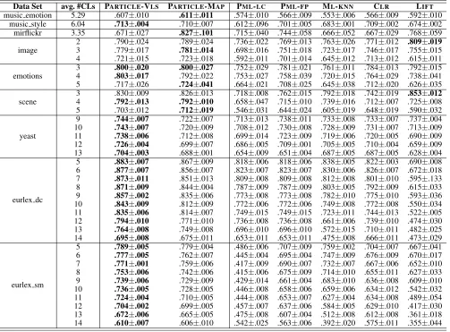
11-Table 4: Experimental results of each comparing approach in terms ofaverage precision, where the best performance (the larger the better) is shown in bold face.
Data Set avg. #CLs PARTICLE-VLS PARTICLE-MAP PML-LC PML-FP ML-KNN CLR LIFT
music emotion 5.29 .607±.010 .611±.011 .574±.010 .566±.009 .553±.006 .566±.009 .592±.010 music style 6.04 .713±.004 .710±.007 .612±.096 .701±.005 .683±.001 .709±.002 .674±.002 mirflickr 3.35 .671±.027 .827±.101 .715±.040 .744±.058 .666±.052 .667±.029 .768±.059
image
2 .790±.024 .789±.024 .736±.022 .769±.013 .763±.026 .771±.012 .809±.019 3 .779±.017 .781±.014 .698±.016 .751±.018 .723±.017 .746±.017 .755±.015 4 .721±.015 .723±.018 .592±.011 .701±.014 .645±.012 .713±.012 .615±.011
emotions
3 .800±.020 .800±.027 .752±.029 .781±.021 .761±.011 .784±.013 .792±.015 4 .803±.017 .792±.022 .753±.027 .758±.039 .720±.015 .764±.029 .738±.041 5 .717±.026 .724±.041 .664±.021 .708±.025 .645±.038 .712±.020 .626±.035
scene
3 .830±.009 .826±.013 .718±.008 .762±.015 .792±.018 .742±.019 .853±.012 4 .792±.013 .792±.010 .658±.047 .715±.010 .739±.016 .712±.007 .725±.008 5 .703±.012 .712±.019 .546±.031 .644±.024 .605±.019 .648±.019 .590±.032
yeast
9 .744±.007 .722±.007 .713±.013 .738±.011 .733±.008 .733±.007 .737±.004 10 .743±.007 .720±.009 .708±.012 .730±.008 .728±.009 .731±.007 .713±.009 11 .738±.006 .712±.008 .699±.014 .723±.009 .719±.006 .720±.005 .690±.009 12 .726±.004 .699±.007 .686±.005 .709±.001 .705±.005 .710±.004 .659±.009 13 .704±.003 .688±.001 .654±.009 .651±.004 .687±.005 .687±.005 .628±.004
eurlex dc
5 .883±.007 .867±.009 .818±.006 .818±.006 .838±.005 .822±.003 .690±.008 6 .877±.007 .856±.007 .823±.007 .823±.007 .830±.006 .826±.007 .672±.018 7 .873±.011 .851±.013 .809±.008 .809±.008 .812±.008 .801±.010 .595±.133 8 .871±.009 .844±.004 .787±.009 .787±.009 .803±.005 .792±.009 .615±.033 9 .857±.002 .835±.006 .773±.008 .773±.008 .782±.010 .775±.010 .593±.036 10 .843±.009 .812±.009 .772±.006 .772±.006 .749±.008 .772±.008 .550±.034 11 .835±.006 .814±.007 .749±.015 .749±.015 .723±.011 .744±.013 .522±.005 12 .794±.010 .771±.010 .736±.008 .736±.008 .661±.006 .739±.010 .474±.030 13 .764±.008 .749±.008 .696±.010 .696±.010 .572±.015 .710±.011 .482±.025 14 .695±.008 .675±.011 .653±.011 .653±.011 .475±.008 .666±.011 .473±.029
eurlex sm
5 .789±.005 .779±.004 .486±.006 .707±.009 .759±.002 .704±.007 .667±.041 6 .777±.005 .762±.007 .445±.004 .695±.004 .747±.009 .676±.009 .670±.017 7 .771±.001 .759±.006 .417±.009 .690±.007 .732±.007 .667±.006 .652±.010 8 .753±.006 .742±.006 .415±.006 .675±.009 .714±.010 .655±.011 .627±.033 9 .739±.006 .729±.009 .429±.014 .661±.004 .683±.010 .636±.008 .609±.010 10 .736±.005 .728±.005 .446±.008 .658±.006 .659±.006 .634±.012 .542±.032 11 .724±.004 .710±.005 .444±.008 .653±.007 .627±.004 .634±.008 .489±.054 12 .704±.002 .699±.005 .457±.007 .637±.006 .584±.005 .629±.010 .417±.030 13 .672±.006 .665±.005 .475±.008 .607±.004 .512±.008 .612±.008 .361±.018 14 .610±.007 .606±.010 .542±.025 .563±.006 .392±.020 .575±.011 .355±.044
13). In this paper, the two variants of PARTICLEinstantiated with virtual label splitting and MAP reasoning are termed as PARTICLE-VLSand PARTICLE-MAPrespectively.
Experiments
Experimental Setup
Data Sets To thoroughly evaluate the performance of comparing approaches, a number of synthetic as well as real-world PML data sets have been employed for experimental studies. Table 2 summarizes characteristics of the experi-mental data sets used in this paper.
Specifically, a synthetic PML data set is generated from one multi-label data set by adding random labeling noise. For each multi-label example, some of its irrelevant la-bels are randomly chosen to form the candidate label set along with its relevant labels. As shown in Table 2, six benchmark multi-label data sets (Zhang and Zhou 2014) are used to generate synthetic PML data sets, includ-ing image, emotions, scene, yeast, eurlex dc, and eurlex sm. For each multi-label data set,
differ-ent settings are considered by varying the average num-ber of candidate labels (avg. #CLs). Accordingly, a total of thirty-four synthetic PML data sets have been gener-ated. Furthermore, three real-world PML data sets includ-ing music emotion, music style andmirflickr (Huiskes and Lew 2008) are also employed in this paper. For the real-world PML data set, candidate labels are collected from web users which are further examined by human la-bellers to specify the ground-truth labels.
Comparing Approaches Three well-established multi-label learning algorithms ML-KNN(Zhang and Zhou 2007), CLR (F¨urnkranz et al. 2008), and LIFT (Zhang and Wu 2015) are employed as the comparing approaches, which are tailored to learn from PML training examples by treating all candidate labels as ground-truth ones. In addition, two re-cent counterpart PML algorithms named PML-LCand PML
Table 5: Win/tie/loss counts of pairwiset-test (at 0.05 significance level) between PARTICLEand each comparing approach.
Evaluation Metric PARTICLE-VLSagainst PARTICLE-MAPagainst
PML-LC PML-FP ML-KNN CLR LIFT PML-LC PML-FP ML-KNN CLR LIFT
Hamming loss 27/0/10 26/0/11 30/0/7 34/3/0 34/3/0 30/1/6 19/2/16 36/0/1 37/0/0 37/0/0
One-error 36/1/0 37/0/0 37/0/0 36/1/0 35/0/2 36/1/0 37/0/0 33/1/3 30/2/5 32/1/4
Coverage 35/1/1 36/0/1 36/1/0 37/0/0 32/0/5 31/1/5 31/1/5 32/0/5 31/1/5 31/0/6
Ranking loss 34/2/1 31/1/5 35/0/2 35/0/2 30/1/6 35/0/2 32/0/5 32/0/5 33/1/3 32/1/4
Average precision 35/1/1 36/0/1 37/0/0 37/0/0 33/0/4 36/1/0 33/0/4 33/1/3 33/0/4 33/0/4
Total 167/5/13 166/1/18 175/1/9 179/4/2 164/4/17 168/4/13 152/3/30 166/2/17 164/4/17 165/2/18
Parameters suggested in respective literatures are used for the comparing approaches, and Libsvm (Chang and Lin 2011) is used as the base learner to instantiate CLR and LIFT. As shown in Table 1, parametersk(number of near-est neighbors considered),α(balancing parameter) andthr (credible label elicitation threshold) for PARTICLE are set to be 10, 0.95 and 0.9 respectively. Furthermore, Libsvm (Chang and Lin 2011) is also utilized to serve as the binary training algorithmBfor PARTICLE.
Five popular multi-label metricshamming loss,one-error,
coverage,ranking lossandaverage precisionare employed for performance evaluation, whose detailed definitions can be found in (Zhang and Zhou 2014; Gibaja and Ventura 2015). On each data set, five-fold cross-validation is per-formed where the mean metric value as well as standard de-viation are recorded for each comparing approach.
Experimental Results
Tables 3 and 4 report the detailed experimental results of each comparing algorithm in terms ofranking lossand av-erage precision, while similar observations can be made in terms of other evaluation metrics. For each data set and evaluation metric, pairwiset-test based on five-fold cross-validation (at 0.05 significance level) is conducted to show whether the performance of PARTICLEis significantly dif-ferent to the comparing approach. Accordingly, Table 5 sum-marizes the resulting win/tie/loss counts over 37 data sets and 5 evaluation metrics.
Based on the experimental results of comparative studies, it is impressive to observe that:
• Out of 185 statistical tests (37 data sets × 5 evalua-tion metrics), PARTICLE-VLS significantly outperforms the counterpart PML approaches PML-LC and PML-FP
in 90.2% and 89.7% cases, and significantly outperforms the tailored MLL approaches ML-KNN, CLRand LIFTin 94.6%, 96.7% and 94.5% cases.
• Similarly, PARTICLE-MAP significantly outperforms PML-LCand PML-FPin 90.8% and 82.1% cases, and sig-nificantly outperforms ML-KNN, CLRand LIFTin 89.7%, 88.6% and 89.1% cases.
• On the real-world PML data sets music emotion, music style and mirflickr, the two variants of PARTICLE achieve optimal performance in almost all cases (except onmusic stylewhere CLRoutperforms
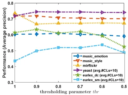
Figure 2: Performance of PARTICLE-VLSchanges as param-eterthrvaries from 1 to 0.5 with an interval of 0.1 (in terms ofaverage precision).
PARTICLEin terms ofranking loss). Furthermore, the per-formance advantage of PARTICLEis more pronounced on synthetic PML data sets with large avg. #CLs (yeast, eurlex dc, andeurlex sm).
As shown in Table 1,thr serves as a crucial parameter which controls the amount of credible labels elicited in the first phase. Figure 2 gives an illustrative example on how the performance of PARTICLE(the virtual label splitting variant) changes as the value of parameterthrvaries. It is shown that the performance of PARTICLEbecomes relatively stable as thrdecrease to 0.9, which is the value used in this paper.
Conclusion
Acknowledgement
The authors wish to thank the anonymous reviewers for their helpful comments and suggestions. This work was supported by the National Key R&D Program of China (2018YFB1004300), the National Science Foundation of China (61573104), the Fundamental Research Funds for the Central Universities (2242018K40082), and partially sup-ported by the Collaborative Innovation Center of Novel Soft-ware Technology and Industrialization.
References
Boutell, M. R.; Luo, J.; Shen, X.; and Brown, C. M. 2004. Learning multi-label scene classification. Pattern Recogni-tion37(9):1757–1771.
Burkhardt, S., and Kramer, S. 2018. Online multi-label dependency topic models for text classification. Machine Learning107(5):859–886.
Chang, C.-C., and Lin, C.-J. 2011. LIBSVM: A library for support vector machines. ACM Transactions on Intelligent Systems and Technology2:27:1–27:27. Software available at http://www.csie.ntu.edu.tw/∼cjlin/libsvm.
Chen, Y.-C.; Patel, V. M.; Chellappa, R.; and Phillips, P. J. 2014. Ambiguously labeled learning using dictionaries.
IEEE Transactios on Information Forensics and Security
9(12):2076–2088.
Chen, C.-H.; Patel, V. M.; and Chellappa, R. 2018. Learning from ambiguously labeled face images. IEEE Transactions on Pattern Analysis and Machine Intelligence40(7):1653– 1667.
Cour, T.; Sapp, B.; and Taskar, B. 2011. Learning from partial labels. Journal of Machine Learning Research
12(May):1501–1536.
F¨urnkranz, J.; H¨ullermeier, E.; Loza Menc´ıa, E.; and Brinker, K. 2008. Multilabel classification via calibrated label ranking. Machine Learning73(2):133–153.
Gibaja, E., and Ventura, S. 2015. A tutorial on multilabel learning.ACM Computing Surveys47(3):Article 52. Gong, C.; Liu, T.; Tang, Y.; Yang, J.; Yang, J.; and Tao, D. 2018. A regularization approach for instance-based su-perset label learning. IEEE Transactions on Cybernetics
48(3):967–978.
Huiskes, M. J., and Lew, M. S. 2008. The mir flickr retrieval evaluation. In Proceedings of the 1st ACM International Conference on Multimedia Information Retrieval, 39–43. Li, Y.; Song, Y.; and Luo, J. 2017. Improving pairwise rank-ing for multi-label image classification. InProceedings of the IEEE Computer Society Conference on Computer Vision and Pattern Recognition, 1837–1845.
Liu, L., and Dietterich, T. 2012. A conditional multino-mial mixture model for superset label learning. In Bartlett, P.; Pereira, F. C. N.; Burges, C. J. C.; Bottou, L.; and Wein-berger, K. Q., eds.,Advances in Neural Information Process-ing Systems 25. Cambridge, MA: MIT Press. 557–565. Read, J.; Pfahringer, B.; Holmes, G.; and Frank, E. 2011. Classifier chains for multi-label classification. Machine Learning85(3):333–359.
Sun, Y.-Y.; Zhang, Y.; and Zhou, Z.-H. 2010. Multi-label learning with weak label. InProceedings of the 24th AAAI Conference on Artificial Intelligence, 593–598.
Tan, Q.; Yu, G.; Domeniconi, C.; Wang, J.; and Zhang, Z. 2018. Multi-view weak-label learning based on matrix com-pletion. InProceedings of the 2018 SIAM International Con-ference on Data Mining, 450–458.
Tsoumakas, G.; Katakis, I.; and Vlahavas, I. 2011. Random k-labelsets for multi-label classification.IEEE Transactions on Knowledge and Data Engineering23(7):1079–1089. Wei, T.; Guo, L.-Z.; Li, Y.-F.; and Gao, W. 2018. Learning safe multi-label prediction for weakly labeled data.Machine Learning107(4):703–725.
Wu, X., and Zhang, M.-L. 2018. Towards enabling binary decomposition for partial label learning. InProceedings of the 27th International Joint Conference on Artificial Intelli-gence, 2868–2974.
Xie, M.-K., and Huang, S.-J. 2018. Partial multi-label learn-ing. InProceedings of the 32nd AAAI Conference on Artifi-cial Intelligence, 4302–4309.
Yu, F., and Zhang, M.-L. 2017. Maximum margin partial label learning. Machine Learning106(4):573–593.
Zhang, M.-L., and Wu, L. 2015. Lift: Multi-label learning with label-specific features. IEEE Transactions on Pattern Analysis and Machine Intelligence37(1):107–120.
Zhang, M. L., and Zhou, Z. H. 2007. Ml-knn: A lazy learn-ing approach to multi-label learnlearn-ing. Pattern Recognition
40(7):2038–2048.
Zhang, M.-L., and Zhou, Z.-H. 2014. A review on multi-label learning algorithms.IEEE Transactions on Knowledge and Data Engineering26(8):1819–1837.
Zhang, M.-L.; Li, Y.-K.; Liu, Y.-Y.; and Geng, X. 2018. Bi-nary relevance for multi-label learning: An overview. Fron-tiers of Computer Science12(2):191–202.
Zhang, M.-L.; Yu, F.; and Tang, C.-Z. 2017. Disambiguation-free partial label learning. IEEE Transac-tions on Knowledge and Data Engineering 29(10):2155– 2167.
Zhou, Z.-H., and Zhang, M.-L. 2017. Multi-label learn-ing. In Sammut, C., and Webb, G. I., eds., Encyclopedia of Machine Learning and Data Mining, 2nd Edition. Berlin: Springer.