Comparison of Classical and Retrial Mx/G/1 Queueing System Under Multiple Adapted Vacation Policy

Comparison of Classical and Retrial M

x

/G/1

Queueing System Under Multiple Adapted

Vacation Policy

M.I.Afthab Begum#1, R.Jayanthidevi#2

#1

Professor, Department of Mathematics, Avinashilingam University, Coimbatore, Tamil Nadu, India

#2

Research Scholar, Department of Mathematics, Avinashilingam University, Coimbatore, Tamil Nadu, India

Abstract –

This paper deals with classical and retrial (MX/G/1) queueing systems in which the breakdown occurs during busy period and sent for repair immediately. The service interrupted customers stay in service facility to complete remaining service for both the models. Further, it is assumed that server takes Multiple Adapted Vacation policy when the system becomes idle. For both the models the system is studied under steady state using Supplementary variable technique. The partial generating function when the system is in different states are calculated. The system size probabilities and the average number of customers waiting in the system when the server is busy or on vacation or in breakdown state are also calculated. The performance measures are presented. The results of both models are compared when 𝑨∗(𝝀) →1. Moreover results of different vacations are presented.

Keywords – Multiple adapted vacation policy, Classical and retrial, Server vacation, Breakdown.

I. INTRODUCTION

In classical queueing models, servers are always available in the service facility. However in many practical situations servers may become unavailable for a period of time due to a variety of reasons. This period of server absence is called server vacation. i.e., vacation in queueing models represents the period of temporary server absence. There are two major types of vacation mechanism, namely exhaustive and non-exhaustive services. With an exhaustive service, the server cannot take a vacation until the system becomes empty. On the other hand non-exhaustive system, the server can take a vacation between two services, during busy period. In either case, the rules for resuming service vacation completion instant are numerous. Based on these rules the two main vacation policies, framed under the exhaustive service discipline are single and multiple vacation policies.

J.C.Ke (2007) introduced the J-vacation policy in which the server can take finite number of vacations (atmost J) during an idle period. Recently Mytalas and Zazanis (2015) introduced the multiple adapted vacation policy in which the server can take decision whether to go for vacation or stay idle in the system at the end of every vacations. It is characterized by a sequence of probabilities and hence generalizes the other vacation policies with the suitable selection of the parameters.

In Retrial queueing systems, a primary customer who does not get service immediately leaves the service area and come back to the system after some period of time and request for service. An arriving customer, encountering the server busy, join a virtual queue called orbit.

Retrial queues play an important role in telephone systems, communication and networking, healthcare, transportation, manufacturing etc. As far as the analytical results are concerned, it is difficult to obtain in retrial queues, but there are great number of numerical and approximation methods. Generally, in queueing systems, the server (human or machine) is subjected to unpredictable breakdowns. As soon as the server breaks down, it will be sent for repair immediately and the system will not work for a short period of time. In the literature of queueing systems with server break downs, two types of behaviours of the customers whose service is interrupted are considered. The first type of behaviour is that, the customers will lose the service completely and will start a new service as soon as the server is fixed. The second behaviour is the customer will stay in the service facility until the server gets repaired and complete the remaining service.

II. MATHEMATICAL ANALYSIS OF THE SYSTEM

A. Model Description

1) Arrival Pattern

The present paper considers an MX/G/1 queueing system in which the arrivals occur in batches in accordance with a time homogeneous Poisson process with random batch size X, group arrival rate λ and probability distribution Pr(X=k)=gk, k=1,2,3… The customers are served one by one according to the order in

the queue.

In case of retrial queues, there is no waiting space in front of the server, therefore, if an arriving batch finds the server idle, then one of the arriving customers begins to receive his service immediately and the others leave the service area and enter into “orbit” according to FCFS queue discipline. The customer at the head of the retrial queue competes with potential primary customers, to decide which customer will enter the next service. If a batch of primary customers arrives first, the retrial customers may cancel its attempt for service and either returns to its position in the retrial queue with probability q or quits the system with probability (1-q).

The retrial time of the customer in the retrial queue is generally distributed with distribution function A(t), density function a(t) and LST A*(θ). Further it is assumed that, the retrial times begin only when the server is freely available in the system (i.e., either at the completion instants of services or vacation completion instants). When the server is idle, arriving (new arrival) customers must turn on the server immediately. If the server is found busy or on vacation or in breakdown state, the arriving batch joins the retrial queue according to FCFS discipline.

2) Multiple Adapted Vacation Policy (MAV)

A cycle starts whenever the system becomes empty and the server is deactivated. The deactivated server either leaves the system for a vacation (first vacation) of random length (VI) with probability β0 or remains idle

in the system with probability (1- β0). Upon returning from the vacation, if the server finds atleast one customer

waiting in the system(classical queues) or orbit(retrial queues), then busy period of the server starts immediately. Otherwise, if there are no customers found waiting in the queue then the server either joins the system with the probability (1- β1) or takes a new vacation (second vacation) with probability β 1. This pattern

continues until atleast one customer is found in the system. Thus the vacation policy is determined by the sequence of probabilities {βi}, i=0, 1, 2,… (i,e.) The vacations have independent duration with common

distribution function VI(t) and density function vI(t) of finite moments.

3) Busy Period and Breakdown Period

During busy period, the server provides single service. The service times follow general (arbitrary) distributions with distribution functions S(t) and the density functions s(t)of finite moments E(Sk), k=1,2.

The server may breakdown at any time while providing service and the server is sent for repair instantaneously. The service channels will not function for a short interval of time. The service interrupted customer stays in the service facility and server starts the service from where it got interrupted. The breakdowns occur according to the Poisson process with rate α and the repair times (denoted by R) of the server is assumed to be arbitrarily distributed with distribution function R(t), density function r(t) for t≥0.

The customers continue to arrive according to the Compound Poisson process, independent of the state of the system and wait in the queue during the busy period, breakdown period and vacation period. The service completion period of a customer consists of the service time and repair time of the server. Thus a cycle is made up of idle vacation period, busy period and breakdown period.

We denote the model by MX/G/1/MAV/breakdown(Resuming service), where MAV denotes the Multiple Adapted Vacation policy. Various stochastic processes involved in the queueing system are assumed to be independent to each other. Using supplementary variable technique the steady state system equations under the steady state condition are analysed and the PGF of the system size is obtained so that various performance measures of the model can be derived from it.

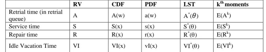
Table 1 : Notations For Analysing The Steady State Results Of The Model

RV CDF PDF LST kth moments

Retrial time (in retrial

queue) A A(w) a(w) A

*

(

𝜃

Service time S S(x) s(x) S*() E(Sk)

Repair time R R(x) r(x) R*() E(Rk)

N (t): The system size at time t

λ : Group arrival rate

X : Group size random variable gk : Pr(X = k), k = 1, 2, 3, …

X(z) : Probability generating function of X.

The notations of Random Variables (RV), Cumulative Distribution Functions (CDF), Probability Density Function (PDF), Laplace-StieltjesTransform (LST) and its kth moments of the RVs are listed in Table (1).

If f(x) is the density function of the probability distribution F(x) then

F∗ _{θ = e}∞ −θx

0 f x dx = e

−θx ∞

0 d F x

Let VI0 t , A0 t , S0 t and R0(t) denote the remaining times of the random variables namely Idle vacation time, retrial time, the service time and repair time respectively.

Let the state of the system at time t be given by Y(t) = 0, 1, 2, 3 according as the server is idle in the system, on vacation during idle time, busy state and break down state respectively. The supplementary variables are introduced in order to obtain a bivariate Markov Process {N(t),(t)} where N(t) denotes the system size at time t and δ t = (0, V0 t , S0 t , R0 t ) according as Y (t) = (0, 1, 2, 3) respectively.

Let PI(t) = Pr {Y(t) = 0, N(t) = 0}

QIn,j(x, t) dt = Pr {N(t) = n, x <V°(t) ≤ x + dt, Y(t) = 1} ; n ≥ 0

Pn(x, t) dt = Pr {N(t) = n, x <S°(t) ≤ x + dt, Y(t) = 2} ; n ≥ 1

Bn(x, y, t) dt = Pr {N(t) = n, x <

R



t

In retrial queues the idle state will be PI0(t) = Pr{N(t) = 0, Y(t) = 0} ; n = 0

PIn(t) = Pr{N(t) = n, Y(t) = 0} ; n ≥ 0

PIn(x,t)dt is the joint probability that at time t, there are n customers in the retrial orbit, and the server is

idle and the remaining retrial time of the server is between w and w + dt, where n ≥ 1 and PI0 is the probability

that the server is idle at time t, and there is no customer in the retrial orbit. Other states remain same as in classical queues.

Then, QIn,j(x,t)dt is the joint probability that at time t, there are n customers in the system and the

remaining vacation time of the server is between x and x + dt, where n0.

Pn(x, t) dt is the joint probability that at time t, there are n customers in the system, the server is busy

and the customer being served in the service channel with remaining service time lies between x and x + dt, where n1.

Bn(x, y, t) denotes the probability that there are n-customers in the system at time t, the server is under

repair and the remaining service time for the customer is equal to x, and the server is being repaired with the remaining repair time between y and y + dt.

PI(t) denotes that the server is idle in the empty system at time t.

Assuming that at steady-state, the probabilities are independent of time t we have

lim

t→∞

∂

∂xPn x, t = d

dxPn x ; limt→∞

∂

∂xQIn,j x, t = d

dxQIn,j x lim

t→∞

∂

∂xBn x, y, t = d

dxBn x, y lim

t→∞

∂

∂tPn x, t = ∂

∂tQIn,j x, t = ∂

∂tBn x, y, t = 0

At steady state Pn 0 ,QIn,j 0 , and Bn 0 denote the probability that there are n customers in the system at the

termination of service period,vacation period and repair period respectively.

III. CLASSICAL QUEUES

A. The Steady State System Size Equations

Idle state

λPI = 1 − βj ∞

j=1

QI0,j 0 + P1 0 1 − β0 1

Vacation during idle state

− d

dxQI0,1 x = −λQI0,1 x + P1 0 β0vI x − d

dxQI0,j x = −λQI0,j x + QI0,j−1 0 βj−1vI x , j ≥ 2 − d

dxQIn,j x = −λQIn,j x + QIn−k,j x

n

k=1

gk n ≥ 1, j ≥ 1

Busy state

− d

dxP1 x = − λ + α P1 x +B1 x, 0 + P2 0 s x

+ QI1,j ∞

j=1

0 s x + λPI g1 s(x)

− d

dxPn x = − λ + α Pn x + λ Pn−k x gk n−1

k=1

+Pn+1 0 s x + Bn x, 0 + QIn,j ∞

j=1

0 s x + λPI gns x , n ≥ 2

Breakdown state

− ∂

∂xB1 x, y = − λB1 x, y + αP1(x) r y

− ∂

∂xBn x, y = − λBn x, y + λ Bn−k

∞

k=1

x, y r y gk + α Pn(x) r y , n ≥ 2

The LST of the above equations are obtained by using the definition of Laplace-Stieltjes transformation and its properties. Thus the LST of the steady -state equations w.r. to x and y are respectively given by:

θQI0,1∗ θ − QI0,1 0 = λQI0,1∗ θ − P1 0 β0VI∗ θ (2)

θQI0,j∗ θ − QI0,j 0 = λQIn,j∗ θ −QI0,j−1 0 βj−1VI∗ θ , j ≥ 2 (3)

θQIn,j∗ θ − QIn,j 0 = λQI0,j∗ θ − λ QIn−k,j∗ θ n

k=1

gk , n ≥ 1 and j ≥ 2 (4)

θP1∗ θ − P1 0 = λ + α P1∗ θ − B1∗ θ, 0

−P2 0 S∗ θ – QI1,j ∞

j=1

0 S∗ _{θ − λ PI g}

1S∗ θ (5)

θPn∗ θ − Pn 0 = λ + α Pn∗ θ − λ Pn−k θ n−1

k=1

gk − Bn∗ θ, 0

−Pn+1 0 S∗ θ − QIn,j ∞

j=1

0 S∗ _{θ − λ PI g}

n S∗ θ , n ≥ 2 6

θ1B∗ ∗ 1 θ, θ1 − B∗ θ, 0 = λ B∗ ∗ 1 θ, θ1 − α Pn∗ θ R∗1 θ1 (7)

θ1B∗ ∗ 1 θ, θ1 − B∗ θ, 0 = λ B∗ ∗ 1 θ, θ1 − α Pn∗ θ R∗1 θ1

−λ Bn−k∗ ∗1 θ, θ1 gk n

k=1

B. Probability Generating Functions

Multiplying the equations (1) to (8) by suitable powers of z and adding, the partial probability generating functions of the system size probabilities at arbitrary epoch when the server is in different states are obtained as shown in equations (9) to (12)

QI∗ _{z, 0 = P} 1 0

1 − VI∗ _w x z

wx z αI0 j ∞

j=0

βi j

i=0

(9)

𝑤ℎ𝑒𝑟𝑒 wx z = λ(1 − X z )

P∗ _{z, 0 =}z P1 0 (−wx z ) I(z)

D(z) hα wx z

1 − S∗ _h

α wx z (10)

where hα wx z = α + wx z − α R∗1( wx z )

I z = 1−VI

∗ _{wx z}

w_x z αI0

j ∞

j=0 ji=0βi+

φ

λ 10.1

D z = z − S∗ _h

α wx z (10.2)

B∗ ∗1 _{z, 0,0 =}α P∗ z, 0 [1 − R∗1 wx z ]

wx z 𝑎𝑛𝑑 (11)

λPI = φP1 0 (12)

where φ = 1 − β∞j=1 j j−1i=0βiαI0jVI∗ wx z + 1 − β0 (13)

The total PGF of the system size distribution is obtained by adding equations (9) to (12) and is given by

P z = P∗ _{z, 0 +B}∗ ∗1 _{z, 0,0 + QI}∗ _{z, 0 + PI}

= P1 0 I z z − 1

S∗ _h

α wx z

D z (14)

C. Stability Condition

Using normalizing condition 1 = lim

z→1P z , we get

P1 0 =

1 − ρ

I(1) (15)

where

,

ρ = 1 + αE R E S λ E X (17)

Substituting for

P

0

P z = 1 − ρ I(1)

I(z)

D(z) S∗ hα (wx z (z − 1) (18)

D. Decomposition Property

The equation (18) can be written as

P z = 1 − ρ (z − 1) I z I 1

S∗ _h

α (wx z

D(z) (19)

The equation (19) shows that the PGF of the system size of the model under consideration is decomposed into the product of two probability generating functions, one of which is the PGF of the single server bulk arrival queuing model with server breakdown without vacation and the other gives the conditional

system size distribution 𝐼 𝑧 _{𝐼 1} during the server idle period under the condition ρ< 1.

IV. RETRIAL QUEUES

A. The Steady State System Size Equations Idle state

λPI0= ∞j=1 1 −βj QI0,j 0 + P0 0 1 −β0 (20)

− d

dwPIn w = −λ PIn w + Pn 0 a w + QIn,j 0 ∞

j=1

a w , n ≥ 1

Vacation during idle state

− d

− d

dxQI0,j x = −λQI0,j x + QI0,j−1 0 βj−1vI x , j ≥ 2

− d

dxQIn,j x = −λQIn,j x + QIn−k,j x

n

k=1

gk , n ≥ 1, j ≥ 1

Busy state

− d

dxP0 x = − λ+α P0 x +B0 x, 0 + PI0 0 s x +λ P1

∞

0

w d w g1 1 − q s x

+λPI0(x) g1 s(x)

− d

dxPn x = − λ+α Pn x +λ Pn−k x gk

n−1

k=1

+PIn+1 0 s x + Bn x, 0 +λPI0 x gn+1s x

+ qλs x PIn−k+1 w dwgk n

k=1

∞

0

+ 1 − q λs x PIn−k+2 w dwgk n+1

k=1

∞

0

,

n ≥ 1

Breakdown state

− ∂

∂yB0 x, y = − λB0 x, y +αP0 x r y

− ∂

∂yBn x, y = − λBn x, y +λ Bn−k

n

k=1

(x, y)gk +αPn x r y , n ≥ 0

The L.S.T of the steady state equations are listed in equations (21) to (28)

θPIn∗ θ − PIn 0 = λPIn∗ θ − Pn 0 A∗ θ − QIn,j 0 A∗ ∞

j=1

θ , n ≥ 1 (21)

θQI0,1∗ θ − QI0,1 0 = λQI0,1∗ θ − P0 0 β0VI∗ θ (22)

θQI0,j∗ θ − QI0,j 0 = λQI0,j∗ θ −QI0,j−1 0 βj−1VI∗ θ , j ≥ 1 (23)

θQIn,j∗ θ − QI𝑛,𝑗 0 = 𝜆𝑄𝐼𝑛,𝑗∗ 𝜃 − 𝜆 𝑄𝐼𝑛−𝑘∗ 𝜃 𝑛

𝑘=1

𝑔𝑘, 𝑗 ≥ 1, 𝑛 ≥ 1 (24)

𝜃𝑃0∗ 𝜃 − 𝑃0 0 = 𝜆 + 𝛼 𝑃0∗ 𝜃 − 𝐵0∗ 𝜃, 0 − 𝑃𝐼1 0 𝑆∗ 𝜃 − 𝜆𝑃𝐼0𝑔1 𝑆∗ 𝜃

− 1 − 𝑞 𝜆 𝑆∗ _{𝜃 𝑃𝐼}

1 𝑤 𝑑𝑤𝑔1 ∞

0

(25) 𝜃𝑃𝑛∗ 𝜃 − 𝑃𝑛 0 = 𝜆 + 𝛼 𝑃𝑛∗ 𝜃 − 𝑃𝐼𝑛+1 0 𝑆∗ 𝜃 − 𝐵𝑛∗ 𝜃, 0 − 𝜆𝑃𝐼0𝑔𝑛+1 𝑆∗ 𝜃

− 𝜆 𝑃𝑛−𝑘∗ 𝜃 𝑛

𝑘=1

𝑔𝑘 − 𝑞𝜆𝑆∗ 𝜃 𝑃𝐼𝑛−𝑘+1 𝑤 𝑑𝑤𝑔𝑘 𝑛

𝑘=1 ∞

0

− 1 − 𝑞 𝜆𝑆∗ _{𝜃 𝑃𝐼}

𝑛−𝑘+2 𝑤 𝑑𝑤𝑔𝑘

𝑛+1

𝑘=1 ∞

0 𝑛 ≥ 1 (26)

𝜃1𝐵0∗∗1 𝜃, 𝜃1 − 𝐵0∗ 𝜃, 0 = 𝜆𝐵0∗∗1 𝜃, 𝜃1 − 𝛼𝑃𝑛∗ 𝜃 𝑅∗1 𝜃1 (27)

𝜃1𝐵𝑛∗∗1 𝜃, 𝜃1 − 𝐵𝑛∗ 𝜃, 0 = 𝜆𝐵𝑛∗∗1 𝜃, 𝜃1 − 𝛼𝑃𝑛∗ 𝜃 𝑅∗1 𝜃1

−𝜆 𝐵𝑛−𝑘∗∗1 𝜃, 𝜃1 𝑛

𝑘=1

𝑔𝑘 𝑛 ≥ 0 (28)

B. Probability Generating Functions

Multiplying the equations (20) to (28) by suitable powers of z and adding, the partial probability generating functions of the system size probabilities at arbitrary epoch when the server is in different states are obtained as shown in equations (29) to (32)

QI∗ _{z, 0 = P} 0 0

1 − VI∗ _w x z

wx z αI0 j ∞

j=0

βi j

i=0

(29)

P∗ _{z, 0 =}P0 0 QR z

hα wx z

1 − S∗ _h

where 𝑄𝑅 𝑍 =

𝑀₁ 𝑧 1−VI∗ _{wx z αI} 0 j ∞

j=0 ji=0βi+φ(X z −𝑀1 𝑧 )

z− S∗ _{hα wx z 𝑀1 𝑧} (30.1) 𝑀1 𝑧 = 𝐴∗ 𝜆 +𝑋 𝑧 _𝑧 1 − 𝑞 − 𝑞𝑧 (1 − 𝐴∗ 𝜆 ) (30.2)

B∗ ∗1 _{z, 0,0 =}α P∗ z, 0 [1 − R∗1 wx z ]

wx z 𝑎𝑛𝑑 (31)

𝑃𝐼∗ _{𝑧, 0 =} 1 − 𝐴∗ 𝜆

𝜆 𝑌1 𝑧 (32) where 𝑌1 𝑧 = 𝑌R 𝑧 P0 0

𝑌R 𝑧 = S∗ hα wx z QR z + 𝑉𝐼∗ 𝑤𝑥 𝑧 − 1 𝛽𝑖𝛼𝐼0𝑗 𝑗

𝑖=0 ∞

𝑗 =0

− φ 32.1

V. COMPARISON

In the present paper the author analyses MX/G/1 classical and retrial queueing model in which the service is subjected to unpredictable breakdown during busy period and takes vacation following Multiple Adapted vacation policy during idle period. Both the models are compared and showed that when 𝐴∗ 𝜆 → 1 the results of both the models coincide.

The probability generating functions given in equations ((9), (10), (11)) are compared with ((29), (30), (31)) when 𝐴∗ 𝜆 → 1 and it is found that the corresponding partial probability generating functions are equal.

VI. PERFORMANCE MEASURES

In this section some useful performance measures of the proposed model are presented.

A. The Steady State System Size Probabilities:

Let PVI , Pbusy and Pbr denote the probability that the server is on vacation, busy state and breakdown

state respectively. Then for classical queues the corresponding probabilities are obtained, by considering the equations in ((9), (10), (11)) at z=1. Thus,

i PVI = lim_z→1QI∗ z, 0 =

1 − ρ

I 1 E(VI) αI0j ∞

j=0

βi j

i=0

ii Pbusy = lim_z→1P∗ z, 0 = λ E X E(S)

iii Pbr = lim_z→1B∗ z, , θ, 0 = α E R Pbusy

and PI =φ

λP1 0 = φ λ

(1 − ρ) I(1)

In retrial queues, PI denote the probability that the server is idle when there are customers in orbit, the corresponding probabilities are obtained, by considering the equations in ((29), (30), (31) and (32)) at z=1

i PVI = lim_z→1QI∗ z, 0 = P0(0)E(VI) αI0j ∞

j=0

βi j

i=0

ii Pbusy = lim_z→1P∗ z, 0 = E(S)QR(1)P0(0)

iii Pbr = lim_z→1B∗ z, , θ, 0 = α E R Pbusy

(iv) 𝑃𝐼 = lim

z→1𝑃𝐼

∗ _{𝑧, 0 =} 1−𝐴∗ 𝜆

𝜆 𝑌𝑅 1 and PI0 = φ λP0(0)

B. Mean System Size

In this section the average number of customers waiting in the system, when the server is in different states are calculated. Let LVI, Lbusy and Lbr denote the expected system size when the server is in vacation

state, busy state and breakdown state respectively. Then the derivatives of equations in (9), (10), (11) at z=1 give the required measures.Thus the mean system size corresponding to different states are given by,

i LVI = _dzd QI∗ z, 0 z=1

=(1 − ρ) I 1

E(VI2₎

2 αI0j ∞

j=0

βi j

i=0

ii Lbusy =

d

dzP∗ z, 0

z=1

=(1 − ρ) I(z)

E X X − 1

2 1 − ρ I 1 E S + λ E X

2 1 − ρ 𝐷′′ 1 E S + λ E X E S I′(1) I(1)

+ [λ E X ]2 _{1 + α E R} E S2

2 + λ E X E S

where −D′′ 1 = S∗ hα (wx z ′′

z=1= λ E X X − 1 E H + λ E X 2 _E(H2₎

and

E H = 1 + α E R E(S)

iii Lbr =

d

dzB∗ z, 0,0

z=1

= α Pbusy λ E X

E R2

2 + Lbusy E R

The total expected system size for the model can be obtained using equation (18)

L = d dzP z

z=1

=I

′ ₁

I 1 + ρ +

−D′′ ₁

2D′ ₁

Then, it is also verified that LVI+ Lbr+ Lbusy = L

In retrial queues, LPI denote the expected system size when the server in idle state the derivatives of

equations in (29), (30), (31) and (32) at z=1 give the required measures.Thus the mean system size corresponding to different states are given by,

i LPI = 1−𝐴

∗ _𝜆

𝜆 𝑌𝑅

′ _{𝑧 P} 0 0

(ii)LVI = P0 0 λE(X)E(VI

2₎

2 αI0

j ∞

j=0 ji=0βi

(𝑖𝑖𝑖)𝐿𝑏𝑢𝑠𝑦 = 𝐸 𝑆 𝑄𝑅′ 1 + 𝜆𝐸 𝑋

𝐸 𝑆2

2 1 + 𝛼𝐸 𝑅 𝑄𝑅 1 P0 0

(iv)Lbr = _dzd B∗ z, 0,0

z=1 = α Pbusy λ E X E R2

2 + Lbusy E R

The total expected system size for the model is L = LPI + LVI+ Lbr+ Lbusy

= P0 0 { 1−𝐴

∗ _𝜆

𝜆 𝑌𝑅

′ _{𝑧 +λE X} E VI2

2 αI0

j ∞

j=0 ji=0βi + 𝐸 𝑆 𝑄𝑅′ 1

+𝜆𝐸 𝑋 𝐸 𝑆₂2 1 + 𝛼𝐸 𝑅 𝑄𝑅 1 +α E S 𝑄𝑅 1 λ E X E R

2

2 + (𝐸 𝑆 𝑄𝑅

′ _{1 + 𝜆𝐸 𝑋} 𝐸 𝑆2

2 1 +

𝛼𝐸 𝑅 𝑄𝑅 1 ) E R }

VII.PARTICULAR CASES

In this section the steady state results of the bulk arrival queueing model are analysed corresponding to single vacation, multiple vacation and J- vacation policies. It is interesting to note from the decomposition property that the total PGF P(z) and the mean queue length L of the model differ from that of other vacation policy models only in the expressions of 𝜑, I(z) and I(1) mentioned earlier. Thus to obtain the total PGF and hence the mean queue length for different vacation policies it is enough to present 𝜑, I(z) and I(1) for the models.

For retrial queueing model corresponding to different vacation policies, it is enough to calculate the expressions of

MAV = ∞j=0αI0j ji=0βi 𝑎𝑛𝑑 φ = 1 − β∞j=1 j j−1i=0βiαI0jVI∗ wx z + 1 − β0

The values of 𝜑, I(z)(for classical queues) and MAV(for retrial queues) for different vacation policies:

A. Single vacation model

When β0= 1, βj= 0 for j ≥ 1 the result for single vacation model are obtained. For this we note that

φ = 𝛼𝐼0

I(z) = 1 − VI

∗ _w x z

wx z +

αI0

MAV= 1

B. Multiple vacation model:

With the selection of βj= 1 for every j ≥ 0. It is found that

φ = 𝟎

I(z) = 1 − VI

∗ _w x z

wx z (1 − αI0)

MAV= _(1−αI1

0)

C. J-vacation model

For this vacation policy β0= 1, βj= p for 1 ≤ j ≤ J − 1 and βj= 0 for j ≥ J . Then

φ = αI0 1 − ρ 1 − αI0p J−1

1 − αI0p + αI0 j_pj−1

I(z) = 1 − αI0p J 1 − αI0p

1 − VI∗ _w x z

wx z +

1

λ αI0 1 − p

1 − αI0p J−1

1 − αI0p + αI0 j_pj−1

MAV= 𝟏 + 1− αI_1−αI0p J

0p

D. Non vacation model

For non vacation model βj= 0 for every j ≥ 0, results are given by

φ = 𝟏 I(z) = −1

𝜆

MAV= 𝟎

VIII. CONCLUSION

In the present work, the author analysed the steady state results for MX/G/1 queueing system of classical and retrial queueing models under Multiple Adapted Vacation policy. The probability generating functions for both the models are obtained and discussed when both will coincide. Performance measures are also presented. The results corresponding to other vacation policies are also deduced for both the models.

REFERENCES

[1] Ke.J.C(2007), Operating characteristic analysis MX_{/G/1 system with a variant vacation policy and balking, Applied Mathematical}

Modelling,31,1321-1337