A Kernel Multiple Change-point Algorithm
via Model Selection
Sylvain Arlot [email protected]
Universit´e Paris-Saclay, Univ. Paris-Sud, CNRS, Inria, Laboratoire de math´ematiques d’Orsay, 91405, Orsay, France.
Alain Celisse [email protected]
Laboratoire de Math´ematiques Paul Painlev´e UMR 8524 CNRS-Universit´e Lille 1
ModalProject-Team
F-59 655 Villeneuve d’Ascq Cedex, France
Zaid Harchaoui [email protected]
Department of Statistics University of Washington Seattle, WA, USA
Editor:Kenji Fukumizu
Abstract
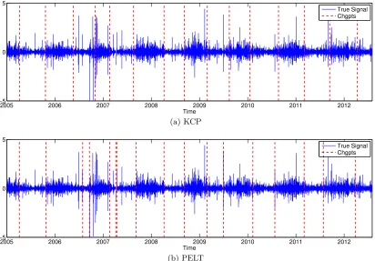
We consider a general formulation of the multiple change-point problem, in which the data is assumed to belong to a set equipped with a positive semidefinite kernel. We propose a model-selection penalty allowing to select the number of change points in Harchaoui and Capp´e’s kernel-based change-point detection method. The model-selection penalty generalizes non-asymptotic model-selection penalties for the change-in-mean problem with univariate data. We prove a non-asymptotic oracle inequality for the resulting kernel-based change-point detection method, whatever the unknown number of change points, thanks to a concentration result for Hilbert-space valued random variables which may be of independent interest. Experiments on synthetic and real data illustrate the proposed method, demonstrating its ability to detect subtle changes in the distribution of data.
Keywords: model selection, kernel methods, change-point detection, concentration in-equality
1. Introduction
The change-point problem has been considered in numerous papers in the statistics and machine learning literature (Brodsky and Darkhovsky, 1993; Carlstein et al., 1994; Tar-takovsky et al., 2014; Truong et al., 2019). Given a time series, the goal is to split it into homogeneous segments, in which the marginal distribution of the observations —their mean or their variance, for instance— is constant. When the number of change points is known, this problem reduces to estimating the change-point locations as precisely as possible; in general, the number of change points itself must be estimated. This problem arises in a wide range of applications, such as bioinformatics (Picard et al., 2005; Curtis et al., 2012), neuroscience (Park et al., 2015), audio signal processing (Wu and Hsieh, 2006), temporal
c
video segmentation (Koprinska and Carrato, 2001), hacker-attacks detection (Wang et al., 2014), social sciences (Kossinets and Watts, 2006) and econometrics (McCulloh, 2009).
1.1. Related Work
A large part of the literature on change-point detection deals with observations in R or Rd and focuses on detecting changes arising in the mean and/or the variance of the signal (Gijbels et al., 1999; Picard et al., 2005; Arlot and Celisse, 2011; Bertin et al., 2017). To this end, parametric models are often involved to derive change-point detection procedures. For instance, Comte and Rozenholc (2004), Lebarbier (2005), Picard et al. (2011) and Geneus et al. (2015) make a Gaussian assumption, while Frick et al. (2014) and Cleynen and Lebarbier (2014) consider an exponential family.
The challenging problem of detecting abrupt changes in the full distribution of the data has been recently addressed in the nonparametric setting. However, the corresponding procedures suffer several limitations since they are limited to real-valued data or they assume that the number of true change points is known. For instance, Zou et al. (2014) design a strategy based on empirical cumulative distribution functions that allows to recover an unknown number of change points by use of BIC, but only applies to R-valued data. The strategy of Matteson and James (2014) applies to multivariate data, but it is time-consuming due to an intensive permutation use, and fully justified only in an asymptotic setting when there is a single change point (Biau et al., 2016). The kernel-based procedure proposed by Harchaoui and Capp´e (2007) enables to deal not only with vectorial data but also with structured data in the sense of G¨artner (2008). The question of model selection, that is the adaptation to unknown number of change points, was raised by Harchaoui and Capp´e (2007, Section 4.1); the present article solves this issue. Finally, many of these procedures cited above were analyzed and justified from a classical asymptotic viewpoint, which may be misleading in particular when the series of datapoints is not long.
Other attempts have been made to design change-point detection procedures allowing to deal with complex data (that are not necessarily vectors). However, the resulting pro-cedures do not allow to detect more than one or two changes arising in particular features of the distribution. For instance, Chen and Zhang (2015) describe a strategy based on a dissimilarity measure between individuals to compute a graph from which a statistical test allows to detect only one or two change points. For a graph-valued time series, Wang et al. (2014) design specific scan statistics to test whether one change arises in the connectivity matrix.
1.2. Main Contributions
Secondly, the procedure (KCP) is theoretically grounded with a finite-sample optimality result, namely an oracle inequality in terms of quadratic risk, stating that its performance is almost the same as that of the best one within the class we consider (Theorem 2). As argued by Lebarbier (2005) for instance, such a guarantee is what we want for a change-point detection procedure. It means that the procedure detects only changes that are “large enough” given the noise level and the amount of data available, which is necessary to avoid having many false positives. A crucial point is that Theorem 2 holds true for any value of the sample sizen; in particular it can be smaller than the dimensionality of the data. Note that contrary to previous oracle inequalities in the change-point detection framework, the result we prove requires neither the variance to be constant nor the data to be Gaussian.
Thirdly, we settle a new concentration inequality for the quadratic norm of sums of independent Hilbert-valued vectors with exponential tails, which is a key result to derive the non-asymptotic oracle inequality for a large collection of candidate segmentations. The exponential concentration inequality may be of independent interest for other statistical problems involving model selection within a large collection of models. Let us finally men-tion that since the first version of the present work (Arlot et al., 2012), KCP has been suc-cessfully applied on different practical examples. Celisse et al. (2018) illustrate that KCP outperforms state-of-the-art approaches on biological data. Cabrieto et al. (2017) show that KCP with a Gaussian kernel outperforms three nonparametric methods for detecting cor-relation changes in synthetic multivariate time series, and provide an application to some data from behavioral sciences. Applying KCP to running empirical correlations (Cabrieto et al., 2018b) or to the autocorrelations of a multivariate time series (Cabrieto et al., 2018a) can make it focus on a specific kind of change —in the covariance between coordinates or in the autocorrelation structure of each coordinate, respectively—, as illustrated on synthetic data experiments and two real-world data sets from psychology.
1.3. Outline and Notation
Motivating examples are first provided in Section 2 to highlight the wide applicability of the procedure to various important settings. A comprehensive description of the proposed kernel change-point detection algorithm (KCP, or Algorithm 1) is provided in Section 3, where we also discuss algorithmic aspects as well as the practical choice of influential parameters (Section 3.3). Section 4 exposes some important ideas underlying KCP and then states the main theoretical results of the paper (Proposition 1 and Theorem 2). Proofs of these main results are collected in Section 5, while technical details are deferred to Appendices A and B. The practical performance of the kernel change-point detection algorithm is illustrated by experiments on synthetic data in Section 6 and on real data in Section 7. Section 8 concludes the paper by a short discussion.
For any a < b, we denote by Ja, bK:= [a, b]∩N the set of integers betweenaand b.
2. The Change-point Problem
Let X be some measurable set and X1, . . . , Xn ∈ X a sequence of independent X-valued
find the locations of the abrupt changes along the sequence PX1, . . . , PXn. Note that the case of dependent time series is often considered in the change-point literature (Lavielle and Moulines, 2000; Bardet and Kammoun, 2008; Bardet et al., 2012; Chang et al., 2018); as a first step, this paper focuses on the independent case for simplicity.
An important example to have in mind is when Xi corresponds to the observation at
timeti =i/nof some random process on [0,1], and we assume that this process is stationary
over [t?`, t?`+1),`= 0, . . . , D?−1, for some fixed sequence 0 =t?0 < t?1 <· · ·< t?D? = 1. Then, the change-point problem is equivalent to localizing the change pointst?1, . . . , t?D?−1∈[0,1], which should be possible as the sample sizentends to infinity. Note that we never make such an asymptotic assumption in the paper, where all theoretical results are non-asymptotic.
Let us now detail some motivating examples of the change-point problem.
Example 1 The set X is R or Rd, and the sequence (PXi)16i6n changes only through its mean. This is the most classical setting, for which numerous methods have been proposed and analyzed in the one-dimensional setting (Comte and Rozenholc, 2004; Zhang and Siegmund, 2007; Boysen et al., 2009; Korostelev and Korosteleva, 2011; Fryzlewicz, 2014) as well as the multi-dimensional case (Picard et al., 2011; Bleakley and Vert, 2011; Hocking et al., 2013; Soh and Chandrasekaran, 2017; Collilieux et al., 2019).
Example 2 The set X is R or Rd, and the sequence (PXi)16i6n changes only through its mean and/or its variance (or covariance matrix). This setting is rather classical, at least in the one-dimensional case, and several methods have been proposed for it (Andreou and Ghysels, 2002; Picard et al., 2005; Fryzlewicz and Subba Rao, 2014; Cabrieto et al., 2017).
Example 3 The set X is R or Rd, and no assumption is made on the changes in the
sequence(PXi)16i6n. For instance, when data are centered and normalized, as in the audio-track example (Rabiner and Sch¨afer, 2007), the mean and the variance of the Xi can be
constant, and only higher-order moments of (PXi)16i6n are changing. Only a few recent papers deal with (an unknown number of ) multiple change points in a fully nonparametric framework: Zou et al. (2014) for X =R, Matteson and James (2014) for X = Rd. Note
that assuming X = R and adding some further restrictions on the maximal order of the
moments for which a change can arise in the sequence(PXi)16i6n, it is nevertheless possible to consider the multivariate sequence ((pj(Xi))06j6d)16i6n, where pj is a polynomial of
degree j for j ∈ {0, . . . , d}, and to use a method made for detecting changes in the mean (Example 1). For instance with R-valued data, as proposed by Lajugie et al. (2014), one
can take pj(X) =Xj for every 16j6d, or pj equal to the j-th Hermite polynomial.
Example 4 The setX is{(p1, . . . , pd)∈[0,1]d such that p1+· · ·+pd= 1}thed-dimensional
simplex. For instance, audio and video data are often represented by histogram features (Oliva and Torralba, 2001; Lowe, 2004; Rabiner and Sch¨afer, 2007), as done in Section 7. In such cases, it is a bad idea to do as if X were Rd-valued, since the Euclidean norm on Rd is usually a bad distance measure between histogram data.
Example 5 The set X is a set of graphs. For instance, the Xi can represent a social
the structure of a time-varying network is a change-point problem. In the case of social networks, this can be used for detecting the rise of an economic crisis (McCulloh, 2009).
Example 6 The set X is a set of texts (strings). For instance, text analysis can try to localize possible changes of authorship within a given text (Chen and Zhang, 2015).
Example 7 The setX is a subset of{A, T, C, G}N, the set of DNA sequences. For instance,
an important question in phylogenetics is to find recombination events from the genome of individuals of a given species (Knowles and Kubatko, 2010; An´e, 2011). This can be achieved from a multiple alignment of DNA sequences (Sch¨olkopf et al., 2004) by detecting abrupt changes (change points) in the phylogenetic tree at each DNA position, that is, by solving a change-point problem.
Example 8 The set X is a set of images. For instance, video-shot boundary detection (Cotsaces et al., 2006) or scene detection in videos (Allen et al., 2017) can be cast as change-point detection problems.
Example 9 The set X is an infinite-dimensional functional space. Such functional data arise in various fields (see for instance Ferraty and Vieu, 2006, Chapter 2), and the problem of testing whether there is a change or not in a functional time series has been considered recently (Ferraty and Vieu, 2006; Berkes et al., 2009; Sharipov et al., 2016).
Other kinds of data could be considered, such as counting data (Cleynen and Lebarbier, 2014; Alaya et al., 2015), qualitative descriptors, as well as composite data, that is, data Xi that are mixing several above examples.
The goal of the paper is to describe a change-point detection procedure that is (i) general enough to handle all these situations (up to the choice of an appropriate similarity measure on X), (ii) in a nonparametric framework, (iii) with an unknown number of change points, and (iv) that can be theoretically analyzed in all these examples simultaneously.
Note also that this procedure is required to output a set of change points that are “close to” the true ones, at least whennis large enough. But in settings where the signal-to-noise ratio is not strong enough to recover all true change points (for a fixed n), false positives are to be avoided. This motivates the non-asymptotic analysis of the procedure based on the (kernel) quadratic risk as a performance measure (see Eq. (9) in Section 4.5). Since the change-point detection procedure relies on model selection, an oracle inequality is proved in Section 4 —Eq. (12) in Theorem 2—, as usually done in non-asymptotic model-selection theory. It establishes that the procedure enjoys a quadratic risk close to the smallest possible value.
3. Detecting Changes in the Distribution With Kernels
3.1. Kernel Change-point Algorithm
For any integerD∈J1, n+ 1K, the set of sequences of (D−1) change points is defined by
TnD :=(τ0, . . . , τD)∈ND+1/0 =τ0< τ1< τ2<· · ·< τD =n (1)
where τ1, . . . , τD−1 are the change points, and τ0, τD are just added for notational
conve-nience. Anyτ ∈ TD
n is called a segmentation (of{1, . . . , n}) intoDτ :=Dsegments.
Let k : X × X → R be a positive semidefinite kernel, that is, a measurable function
X × X → R such that for any x1, . . . , xn ∈ X, the n×n matrix (k(xi, xj))16i,j6n is
positive semidefinite. Examples of such kernels are given in Section 3.2. Then, we measure the quality of any candidate segmentation τ ∈ TD
n with the kernel least-squares criterion
introduced by Harchaoui and Capp´e (2007):
b
Rn(τ) := 1
n
n X
i=1
k(Xi, Xi)−
1 n
D X
`=1
1 τ`−τ`−1
τ`
X
i=τ`−1+1
τ`
X
j=τ`−1+1
k(Xi, Xj)
. (2)
In particular when X =Rand k(x, y) =xy, we recover the usual least-squares criterion
b
Rn(τ) = 1
n
D X
`=1
τ`
X
i=τ`−1+1
Xi−XJτ`−1+1,τ`K
2
where X
Jτ`−1+1,τ`K :=
1 τ`−τ`−1
τ`
X
j=τ`−1+1
Xj.
Note that Eq. (6) in Section 4.1 provides an equivalent formula forRbn(τ), which is helpful
for understanding its meaning. Given the criterion (2), we cast the choice ofτ as a model-selection problem (as thoroughly detailed in Section 4), which leads to Algorithm 1 below, that we now briefly comment on.
Input: observations: X1, . . . , Xn∈ X,
kernel: k:X × X →R,
constants: c1, c2 >0 andDmax∈J1, n−1K.
Step 1: ∀D∈J1, DmaxK, compute (by dynamic programming): b
τ(D)∈argminτ∈TD n
b
Rn(τ) and Rbn bτ(D)
.
Step 2: find:
b
D∈argmin16D6Dmax
b
Rn τb(D)
+ 1 n
c1log
n−1 D−1
+c2D
.
Output: sequence of change points: bτ =bτ Db
.
Algorithm 1: Kernel change-point algorithm (KCP)
• Step 1 of KCP consists in choosing the “best” segmentation with D segments — that is, the minimizer of the kernel least-squares criterionRbn(·) overTnD—, for every
• Step 2 of KCP chooses D by model selection, using a penalized empirical criterion. A major contribution of this paper lies in the building and theoretical justification of the penaltyn−1[c1log Dn−−11
+c2D], see Sections 4–5; a simplified penalty, of the form
D
n(c1log( n
D) +c2), would also be possible, see Section 4.5.
• Practical issues (computational complexity and choice of constants c1, c2, Dmax) are discussed in Section 3.3. Let us only emphasize here that KCP is computationally tractable; its most expensive part is the minimization problem of Step 1, which can be done by dynamic programming (see Harchaoui and Capp´e, 2007; Celisse et al., 2018). Efficient implementations of KCP in Python can be found in the ruptures package (Truong et al., 2018) and in the Chapydette package (Jones and Harchaoui, 2019).
3.2. Examples of Kernels
KCP can be used with various sets X (not necessarily vector spaces) as long as a positive semidefinite kernel on X is available. An important issue is to design relevant kernels, that are able to capture important features of the data for a given change-point problem, including non-vectorial data —for instance, simplicial data (histograms), texts or graphs (networks), see Section 2. The question of choosing a kernel is discussed in Section 8.2.
Classical kernels can be found in the books by Sch¨olkopf and Smola (2001), Shawe-Taylor and Cristianini (2004) and Sch¨olkopf et al. (2004) for instance. Let us mention a few of them:
• WhenX =Rd,klin(x, y) =hx, yiRd defines the linear kernel. When d= 1, KCP then coincides with the algorithm proposed by Lebarbier (2005).
• When X = Rd, khG(x, y) = exp[− kx−yk
2/(2h2)] defines the Gaussian kernel with bandwidth h >0, which is used in the experiments of Section 6.
• WhenX =Rd,khL(x, y) = exp[−kx−yk/h] defines theLaplace kernelwith bandwidth
h >0.
• When X =Rd,keh(x, y) = exp(hx, yiRd/h) defines the exponential kernel with
band-width h > 0. Note that, unlike the Gaussian and Laplace kernels, the exponential kernel is not translation invariant.
• When X = R, kHh(x, y) =
P5
j=1Hj,h(x)Hj,h(y), corresponds to the Hermite kernel,
whereHj,h(x) = 2j+1
√
πj!e−x2/(2h2)(−1)je−x2/2(∂/∂x)j(e−x2/2) denotes thej-th Her-mite function with bandwidthh >0. This kernel is used in Section 6. It can of course be generalized to maximal-degree values different from 5.
• When X is the d-dimensional simplex as in Example 4, the χ2 kernel can be defined by khχ2(x, y) = exp
−h1·dPdi=1(xi−yi)2
xi+yi
for some bandwidth h > 0. An illustration of its behavior is provided in the simulation experiments of Sections 6 and 7.
closeness between points. The so-called energy distance between probability measures is an example (Matteson and James, 2014). In addition, specific kernels have been designed for various kinds of structured data, including all the examples of Section 2 (Cuturi et al., 2005; Rakotomamonjy and Canu, 2005; Shervashidze, 2012; Vedaldi and Zisserman, 2012). Convolutional kernels can also be designed to mimic the feature maps defined by convolu-tional networks, with successful applications in computer vision (Mairal et al., 2014; Paulin et al., 2017).
Let us finally remark that KCP can also be used when k is not a positive semidefinite kernel; its computational complexity remains unchanged, but we might loose the theoretical guarantees of Section 4.
3.3. Practical Issues
Let us now discuss the main practical issues when applying KCP.
3.3.1. Computational Complexity
The discrete optimization problem at Step 1 of KCP is apparently hard to solve since, for each D, there are Dn−−11
segmentations of {1, . . . , n} into D segments. Fortunately, as shown by Harchaoui and Capp´e (2007), this optimization problem can be solved efficiently by dynamic programming. In the special case of a linear kernel, we recover the classical dynamic-programming algorithm for detecting changes in mean (Fisher, 1958; Auger and Lawrence, 1989; Kay, 1993).
Denoting byCkthe cost of computingk(x, y) for some givenx, y∈ X, the computational
cost of a naive implementation of Step 1 —computing each coefficient (i, j) of the cost matrix independently— then isO(Ckn2+Dmaxn4) in time andO(Dmaxn+n2) in space. The computational complexity can actually beO((Ck+Dmax)n2) in time andO(Dmaxn) in space as soon as one either uses the summed area table or integral image technique as in (Potapov et al., 2014) or optimizes the interplay of the dynamic-programming recursions and cost-matrix computations (Celisse et al., 2018). For given constants Dmax and c1, c2, Step 2 is straightforward since it consists in a minimization problem among Dmax terms already stored in memory. Therefore, the overall complexity of KCP is at most O((Ck+Dmax)n2) in time andO(Dmaxn) in space.
3.3.2. Setting the Constants c1 and c2
3.3.3. Setting the Constant Dmax
KCP requires to specify the maximal dimension Dmax of the segmentations considered, a choice that has three main consequences. First, the computational complexity of KCP is affine inDmax, as discussed above. Second, ifDmax is too small —smaller than the number of true change points that can be detected—, the segmentationbτ provided by the algorithm
will necessarily be too coarse. Third, when the slope heuristics is used for choosing c1, c2, taking Dmax larger than the true number of change points might not be sufficient: better values for c1, c2 can be obtained by takingDmax larger, up to n. From our experiments, it seems thatDmax≈n/√logn is large enough to provide good results.
3.4. Related Change-point Algorithms
In addition to the references given in the Introduction, let us mention a few change-point algorithms to which KCP is more closely related.
First, some two-sample (or homogeneity) tests based on kernels have been suggested. They tackle a simpler problem than the general change-point problem described in Section 2. Among them, Gretton et al. (2012a) propose a two-sample test based on a U-statistic of order two, called the maximum mean discrepancy (MMD). A related family of two-sample tests, called B-tests, is proposed by Zaremba et al. (2013); B-tests are also used by Li et al. (2015, 2019) for localizing a single change point. Harchaoui et al. (2008) propose a studentized kernel-based test statistic for testing homogeneity. Resampling methods — (block) bootstrap and permutations— have also been proposed for choosing the threshold of several kernel two-sample tests (Fromont et al., 2012; Chwialkowski et al., 2014; Sharipov et al., 2016).
Second, Harchaoui and Capp´e (2007) consider a kernel-based method for multiple change-point detection, focusing on the case where the true number of segmentsD?is known. Step 1 of KCP builds off the method of Harchaoui and Capp´e (2007). The present paper proposes a data-driven choice ofD supported by non-asymptotic theoretical guarantees.
Third, whenX =Randk(x, y) =xy,Rbn(τ) is the usual least-squares risk and Step 2 of
KCP is similar to the penalization procedures proposed by Comte and Rozenholc (2004) and Lebarbier (2005) for detecting changes in the mean of a one-dimensional signal. We refer readers familiar with model-selection techniques to Section 4.1 for an equivalent formulation of KCP —in more abstract terms— that clearly emphasizes the links between KCP and these penalization procedures.
4. Theoretical Analysis
We now provide theoretical guarantees for KCP. We start by reformulating it in an abstract way, which enlightens how it works.
4.1. Abstract Formulation of KCP
semidefinite kernels and related notions can be found in several books (Sch¨olkopf and Smola, 2001; Cucker and Zhou, 2007; Steinwart and Christmann, 2008).
Let us define Yi = Φ(Xi) ∈ H for every i∈ {1, . . . , n},Y = (Yi)16i6n ∈ Hn, the set of
segmentationsTn:=SnD=1TD
n whereTnD is defined by Eq. (1), and for every τ ∈ Tn,
Fτ :=
f = (f1, . . . , fn)∈ Hn s.t. fτ`−1+1 =· · ·=fτ` ∀16`6Dτ , (3)
which is a linear subspace of Hn. We also define on Hn the canonical scalar product by
hf, gi:=Pni=1hfi, giiHforf, g∈ Hn, and we denote byk·kthe corresponding norm. Then,
for any g∈ Hn,
Πτg:= argminf∈Fτ
n
kf−gk2o (4)
is the orthogonal projection of g∈ Hn onto F
τ, and satisfies
∀g∈ Hn,∀16`6D
τ,∀i∈Jτ`−1+ 1, τ`K, (Πτg)i=
1 τ`−τ`−1
τ`
X
j=τ`−1+1
gj. (5)
This statement is proved in Appendix A.1.
Following Harchaoui and Capp´e (2007), the empirical risk Rbn(τ) defined by Eq. (2) can
be rewritten as
b
Rn(τ) = 1
nkY −µbτk
2 where
b
µτ = ΠτY , (6)
as proved in Appendix A.1.
For each D ∈ J1, DmaxK, Step 1 of KCP consists in finding a segmentation τb(D) in D
segments such that
b
τ(D)∈argminτ∈TD n
n
Y −µbτ
2o
= argminτ∈TD n
(
inf
f∈Fτ
n X
i=1
Φ(Xi)−fi
2
)
,
which is the “kernelized” version of the classical least-squares change-point algorithm (Lebar-bier, 2005). Since the penalized criterion of Step 2 is similar to that of Comte and Rozenholc (2004) and Lebarbier (2005), we can see KCP as a “kernelization” of these penalized least-squares change-point procedures.
Let us emphasize that building a theoretically-grounded penalty for such a kernel least-squares change-point algorithm is not straightforward. For instance, we cannot apply the model-selection results by Birg´e and Massart (2001) that were used by Comte and Rozen-holc (2004) and Lebarbier (2005). Indeed, a Gaussian homoscedastic assumption is not realistic for general Hilbert-valued data, and we have to consider possibly heteroscedastic data for which we assume only that Yi = Φ(Xi) is bounded in H —see Assumption (Db)
in Section 4.3. Note that unbounded data Xi can satisfy Assumption (Db), for instance
4.2. Intuitive Analysis
Section 4.1 shows that KCP can be seen as a kernelization of change-point algorithms focusing on changes of the mean of the signal (Lebarbier, 2005, for instance). Therefore, KCP is looking for changes in the “mean” of Yi = Φ(Xi)∈ H, provided that such a notion
can be defined.
If His separable and E[pk(Xi, Xi)]<+∞, we can define the (Bochner) mean µ?i ∈ H
of Φ(Xi) (Ledoux and Talagrand, 1991), also called the mean element of PXi, by
∀g∈ H, hµ?i, giH =Eg(Xi)
=EhYi, giH
. (7)
Then, we can write
∀16i6n, Yi =µ?i +εi∈ H where εi:=Yi−µ?i .
The variables (εi)16i6n are independent and centered —that is, ∀g ∈ H, E[hεi, giH] = 0.
So, we can understandµbτ as the least-squares estimator overFτ ofµ?= (µ?1, . . . , µ?n)∈ Hn.
An interesting case is whenkis acharacteristic kernel (Fukumizu et al., 2008), or equiv-alently, when Hk is probability-determining (Fukumizu et al., 2004a,b). Then any change
in the distribution PXi induces a change in the mean element µ
?
i. In such settings, we can
expect KCP to be able to detectany changein the distributionPXi, at least asymptotically. For instance the Gaussian kernel is characteristic (Fukumizu et al., 2004b, Theorem 4), and general sufficient conditions for k to be characteristic are known (Sriperumbudur et al., 2010, 2011).
Note that Sharipov et al. (2016) suggest to use k6(x, y) =1x6y as a “kernel” within a
two-sample test, in order to look for any change of the distribution of real-valued dataXi
(Example 3). This idea is similar to our proposal of using KCP with a characteristic kernel for tackling Example 3, even if we do not advise to takek=k6 within KCP. Indeed, when k=k6,Rbn(τ) = 12 −D2nτ as soon as the Xi are all different so that KCP becomes useless.
This illustrates that using a kernel which is not symmetric positive definite should be done cautiously.
4.3. Notation and Assumptions
Throughout the paper, we assume thatHis separable, which is kind of a minimal assumption for two reasons: it allows to define the mean element —see Eq. (7)—, and most reasonable examples satisfy this requirement (Dieuleveut and Bach, 2014, p. 4). Let us further assume
∃M ∈(0,+∞), ∀i∈ {1, . . . , n}, kYik2H =kΦ(Xi)k2H =k(Xi, Xi)6M2 a.s. (Db)
For every 16i6n, we also define the “variance” ofYi by
vi:=E
h
Φ(Xi)−µ?i
2
H
i
=Ek(Xi, Xi)
−µ?i
2
H=E
k(Xi, Xi)−k(Xi, Xi0)
(8)
where Xi0 is an independent copy of Xi, and vmax := max16i6nvi. Let us make a few
remarks.
• If (Db) holds true, then the mean element µ?i exists since E[pk(Xi, Xi)] < ∞, the
• If (Db) holds true, then Yi admits a covariance operator Σi that is trace-class and
vi= tr(Σi).
• If k is translation invariant, that is,X is a vector space and k(x, x0) = k(x−x0) for everyx, x0∈ X, and some measurable functionk:X →R, then (Db) holds true with M2=k(0) andvi =k(0)− kµ?ik2H. For instance the Gaussian and Laplace kernels are
translation invariant (see Section 3.2).
• Let us consider the case of the linear kernel (x, y)7→ hx, yi on X =Rd. If we assume E[kXik2
Rd] < ∞, then, vi = tr(Σi) where Σi is the covariance matrix of Xi. In
addition, (Db) holds true if and only ifkXikRd 6M a.s. for alli.
4.4. Concentration Inequality for Some Quadratic Form of Hilbert-valued Random Variables
Our main theoretical result, stated in Section 4.5, relies on two concentration inequalities for some linear and quadratic functionals of Hilbert-valued vectors. Here we state the concentration result that we prove for the quadratic term, which is significantly different from existing results and can be of independent interest.
Proposition 1 (Concentration of the quadratic term) Let τ ∈ Tn and recall thatΠτ
is the orthogonal projection ontoFτ inHndefined by Eq.(4). LetX1, . . . , Xnbe independent
X-valued random variables and assume that (Db) holds true, so thatε= (ε1, . . . , εn)∈ Hn
is defined as in Section 4.1. Then for everyx >0, with probability at least 1−e−x,
kΠτεk2−EkΠτεk2
6 14M
2 3
x+ 2p2xDτ
.
Proposition 1 is proved in Section 5.4. The proof relies on a combination of Bernstein’s and Pinelis-Sakhanenko’s inequalities. Note that the proof of Proposition 1 also shows that for everyx >0, with probability at least 1−e−x,
kΠτεk2−EkΠτεk2
> −14M
2 3
x+ 2p2xDτ
.
Previous concentration results for quantities such as kΠτεk2 or kΠτεk do not imply
Proposition 1 —even up to numerical constants. Indeed, they either assume that ε is a Gaussian vector, or they involve much larger deviation terms (see Section 5.4.3 for a detailed discussion of these results).
4.5. Oracle Inequality for KCP
Similarly to the results of Comte and Rozenholc (2004) and Lebarbier (2005) in the one-dimensional case, we state below a non-asymptotic oracle inequality for KCP. First, we define the (kernel) quadratic risk of any µ∈ Hnas an estimator of µ? by
R(µ) = 1
nkµ−µ
?k2= 1 n
n X
i=1
Theorem 2 We consider the framework and notation introduced in Sections 2–4. Let C > 0 be some constant. Assume that (Db) holds true and that pen : Tn → R is some
penalty function satisfying
∀τ ∈ Tn, pen(τ)> CM
2 n
log
n−1 Dτ−1
+Dτ
. (10)
Then, some numerical constantL1 >0 exists such that the following holds: if C >L1, for every y>0, an event of probability at least 1−e−y exists on which, for every
b
τ ∈argminτ∈Tn
n
b
Rn(τ) + pen(τ)o , (11)
we have
R(µbbτ)62 inf
τ∈Tn
R(bµτ) + pen(τ) +
83yM2
n . (12)
Theorem 2 is proved in Section 5.5.
Theorem 2 applies to the segmentationτboutput by KCP whenc1 andc2are larger than L1M2. It shows thatµbτbestimates well the “mean” µ
?∈ Hn of the transformed time series
Y1 = Φ(X1), . . . , Yn = Φ(Xn). Such an oracle inequality, namely Eq. (12), is the classical
means for theoretically validating any model-selection procedure in a non-asymptotic way (Birg´e and Massart, 2001, for instance). Since the present change-point detection procedure (KCP) is based on model selection, Eq. (12) can serve as theoretical validation. In addition, such a non-asymptotic optimality result is necessary for taking into account situations where some changes are too small to be detected —they are “below the noise level” (Lebarbier, 2005, for instance). By defining the performance of bτ as the quadratic risk of µbbτ (seen as
an estimator ofµ?), the oracle inequality (12) proves that KCP works well for finite sample size and for a set X that can have a large dimensionality (possibly much larger than the sample sizen). The consistency of KCP for estimating the change-point locations, which is outside the scope of this paper, is discussed in Section 8.1.
Why is a penalty satisfying Eq. (10) a good choice? As detailed in Section 5.1, the oracle inequality in Eq. (12) results from taking a penalty such that, for every τ ∈ Tn,
the (penalized) empirical criterion Rbn(τ) + pen(τ) in Eq. (11) approximates the (oracle)
performance measure R(µbτ). At least, the penalty must be large enough so that
b
Rn(τ) + pen(τ)>R(µbτ)
holds true simultaneously for all τ ∈ Tn (up to technical details exposed in Section 5).
Then, the core of the proof of Theorem 2 is to show that Eq. (10) implies that such a set of inequalities holds true on an event of high probability.
The constant 2 in front of the first term in Eq. (12) has no special meaning, and could be replaced by any quantity strictly larger than 1, at the price of enlarging 83 in the right-hand side of Eq. (12) and the constant L1.
probably are not optimal. Second, the constant M2 in the penalty is probably pessimistic in several frameworks. For instance, with the linear kernel and Gaussian data belonging to
X =R, (Db) is not satisfied, but other similar oracle inequalities have been proved withM2 replaced by the residual variance (Lebarbier, 2005). In practice, as we do in the experiments of Sections 6–7, we recommend to use a data-driven value for the leading constantC in the penalty, as explained in Section 3.3.
Theorem 2 also applies to KCP with simplified penalty shapes. Indeed,
∀D∈ {1, . . . , n},
n−1 D−1
= D n
n D
6
n D
6 n
D
D! 6
ne
D
D
so that Theorem 2 applies to the penalty Dn[c1log(Dn) +c2] —similar to the one of Lebarbier (2005)— as soon as c1, c2 > L1M2. A BIC-type penalty CDlog(n)/n is also covered by Theorem 2 provided that C>2.5L1M2 and n>2, even if we do not recommend to use it —see Section 6.3.
A nice feature of Theorem 2 is that it holds under mild assumptions: we only need the data Xi to be independent and to have (Db) satisfied. As noticed in Section 4.3, (Db)
holds true for any translation-invariant kernel, such as the Gaussian and Laplace kernels. Compared to previous results (Comte and Rozenholc, 2004; Lebarbier, 2005), we do not need the data to be Gaussian or homoscedastic. Furthermore, the independence assumption can certainly be relaxed: to do so, it would be sufficient to prove concentration inequalities similar to Propositions 1 and 3 for some dependent Xi.
In the particular setting whereX =Randkis the linear kernel (x, y)7→xy, Theorem 2 provides an oracle inequality similar to the one proved by Lebarbier (2005) for Gaussian and homoscedastic real-valued data. The price to pay for extending this result to heteroscedastic Hilbert-valued data is rather mild: we only assume (Db) and replace the residual variance by M2.
Apart from the results already mentioned, a few oracle inequalities have been proved for change-point procedures, for real-valued data with a multiplicative penalty (Baraud et al., 2009), for discrete data (Akakpo, 2011), for counting data with a total-variation penalty (Alaya et al., 2015), for counting data with a penalized maximum-likelihood procedure (Cleynen and Lebarbier, 2014) and for data distributed according to an exponential family (Cleynen and Lebarbier, 2017). Among these oracle inequalities, only the result by Akakpo (2011) is more precise than Theorem 2 —there is no log(n) factor compared to the oracle loss—, at the price of using a smaller (dyadic) collection of possible segmentations, hence a worse oracle performance in general.
5. Main Proofs
We now prove the main results of the paper, Theorem 2 and Proposition 1.
5.1. Outline of the Proof of Theorem 2
As usual for proving an oracle inequality (see Arlot, 2014, Section 2.2), we remark that by Eq. (11), for everyτ ∈ Tn,
b
Therefore,
R(µbτb) + pen(bτ)−penid(bτ)6R(µbτ) + pen(τ)−penid(τ) (13)
where ∀τ ∈ T, penid(τ) :=R(µbτ)−Rbn(τ) +
1 nkεk
2 . (14)
The idea of the proof is that if we prove that pen(τ)> penid(τ) for every τ ∈ Tn, we get an oracle inequality similar to Eq. (12). What remains to obtain is a deterministic upper bound on theideal penalty penid(τ) that holds true simultaneously for allτ ∈ Tnon a large
probability event. To this aim, we computeE[penid(τ)] and show that penid(τ) concentrates around its expectation for every τ ∈ Tn (Sections 5.2–5.4). Then we use a union bound as
detailed in Section 5.5. A similar strategy is used for instance by Comte and Rozenholc (2004) and Lebarbier (2005) in the specific context of change-point detection.
Note that we prove below a slightly weaker result than pen(τ) > penid(τ), which is nevertheless sufficient to obtain Eq. (12). Remark also that Eq. (13) would be true if the constantn−1kεk2 in the definition (14) of penidwas replaced by any quantity independent from τ; the reasons for this specific choice appear in the computations below.
5.2. Computation of the Ideal Penalty
From Eq. (14) it results that for everyτ ∈ Tn,
n×penid(τ) =kµbτ−µ?k2− kµbτ−Yk
2+kεk2 =kµbτ−µ?k2− kµbτ−µ
?−εk2
+kεk2
= 2hµbτ−µ?, εi
= 2
Πτ(µ?+ε)−µ?, ε
= 2hΠτµ?−µ?, εi+ 2hΠτε, εi
= 2hΠτµ?−µ?, εi+ 2kΠτεk2 (15)
since Πτ is an orthogonal projection. The next two sections focus separately on the two
terms appearing in Eq. (15).
5.3. Concentration of the Linear Term
We prove in Section A.2 the following concentration inequality for the linear term in Eq. (15), mostly by applying Bernstein’s inequality.
Proposition 3 (Concentration of the linear term) If (Db)holds true, then for every x >0, with probability at least 1−2e−x,
∀θ >0,
(I−Πτ)µ?,Φ(X)−µ?
6θkΠτµ
?−µ?k2+
vmax 2θ +
4M2 3
x . (16)
5.4. Dealing With the Quadratic Term
5.4.1. Preliminary Computations
We start by providing a useful closed-form formula forkΠτεk2 and by computing its
expec-tation. First, a straightforward consequence of Eq. (5) is that
kΠτεk2 =
Dτ X `=1 1 τ`−τ`−1
τ` X
i=τ`−1+1
εi 2 H (17) = Dτ X `=1 " 1 τ`−τ`−1
X
τ`−1+16i,j6τ`
hεi, εjiH
#
. (18)
Second, we remark that for every i, j∈ {1, . . . , n},
Ehεi, εjiH
=EhΦ(Xi),Φ(Xj)iH
−Ehµ?i,Φ(Xj)iH
−E
h
Φ(Xi), µ?j
H
i
+µ?i, µ?jH
=EhΦ(Xi),Φ(Xj)iH
−
µ?i, µ?jH
=1i=j
E[k(Xi, Xi)]− kµ?ik
2
H
=1i=jvi. (19)
Combining Eq. (18) and (19), we get
E
h
kΠτεk2
i = Dτ X `=1 1 τ`−τ`−1
τ`
X
i=τ`−1+1
vi = Dτ X `=1
v`τ, (20)
wherevτ ` :=
1
τ`−τ`−1
Pτ`
i=τ`−1+1vi.
5.4.2. Concentration: Proof of Proposition 1
This proof is inspired from that of a concentration inequality by Sauv´e (2009) in the context of regression with real-valued non-Gaussian noise. Let us define
T`:=
1 τ`−τ`−1
τ` X
j=τ`−1+1
εj 2 H
, so that kΠτεk2 = X
16`6Dτ T`
by Eq. (17). Since the real random variables (T`)16`6Dτ are independent, we get a con-centration inequality for their sum kΠτεk2 via Bernstein’s inequality (Proposition 6 in
Appendix B.1) as long as T` satisfies some moment conditions. The rest of the proof
con-sists in showing such moment bounds by using Pinelis-Sakhanenko’s deviation inequality (Proposition 7 in Appendix B.1).
First, note that (Db) implies thatkεikH 62M almost surely for every i by Lemma 5,
hence kPτ`
i=τ`−1+1εikH 62(τ`−τ`−1)M a.s. for every 16` 6Dτ. Then for every q > 2
and 16`6Dτ,
ET`q= 1 (τ`−τ`−1)q
Z 2(τ`−τ`−1)M
0
2qx2q−1P
τ` X
i=τ`−1+1 εi H >x
Second, since kεikH 6 2M almost surely and E
kεik2H
=vi 6M2 for every i, we get
that for every p>2 and 16`6Dτ,
τ`
X
i=τ`−1+1
EkεikpH
6 p!
2
τ`
X
j=τ`−1+1
vj 2M 3
p−2
6 p!
2 ×(τ`−τ`−1)M 2×
2M 3
p−2
.
Hence, the assumptions of Pinelis-Sakhanenko’s deviation inequality (Pinelis and Sakha-nenko, 1986) —which is recalled by Proposition 7 in Appendix B.1— are satisfied with c= 2M/3 andσ2 = (τ`−τ`−1)M2, and we get that for every x∈[0, 2(τ`−τ`−1)M]
P τ` X
i=τ`−1+1
εi H >x
62 exp −
x2
2(τ`−τ`−1)M2+2M x3
!
62 exp
− 3x
2 14(τ`−τ`−1)M2
.
Together with Eq. (21), we obtain that
ET`q6 4q (τ`−τ`−1)q
Z 2(τ`−τ`−1)M
0
x2q−1exp
− 3x
2 14(τ`−τ`−1)M2
dx
64q
7M2 3
qZ +∞
0
u2q−1exp
−u 2 2 du
= 2q−1(q−1)!×4q
7M2 3
q
= 2×(q!)
14M2 3
q
, (22)
since for everyq >1,
Z +∞
0
u2q−1exp(−u2/2) du= 2q−1(q−1)!. Finally, summing Eq. (22) over 16`6Dτ, it comes
X
16`6Dτ
ET`q62×(q!)
14M2 3
q
Dτ
= q! 2 ×Dτ
28M2 3
2
×
14M2 3
q−2
.
Then, condition (34) of Bernstein’s inequality holds true with
v=Dτ
28M2 3
2
and c= 14M 2
3 .
1−e−x,
kΠτεk2−E
h
kΠτεk2
i
6√2vx+cx
=p2Dτx
28M2
3 +
14M2
3 x
= 14M 2 3
2p2Dτx+x
.
5.4.3. Why Do We Need a New Concentration Inequality?
We now review previous concentration results for quantities such as kΠτεk2 or kΠτεk,
showing that they are not sufficient for our needs, hence requiring a new result such as Proposition 1.
First, when ε ∈ Rn is a Gaussian isotropic vector, kΠ
τεk2 is a chi-square random
variable for which concentration tools have been developed. Such results are used by Birg´e and Massart (2001) and by Lebarbier (2005) for instance. They cannot be applied here sinceεcannot be assumed Gaussian, and theεj do not necessarily have the same variance.
Second, Eq. (18) shows that kΠτεk2 is a U-statistic of order 2. Some tight exponential
concentration inequalities exist for such quantities when εj ∈ R (Houdr´e and Reynaud-Bouret, 2003) and when εj belongs to a general measurable set (Gin´e and Nickl, 2016,
Theorem 3.4.8). In both results, a term of orderM2x2 appears in the deviations, which is too large because the proof of Theorem 2 relies on Proposition 1 with x Dτ: we really
need a smaller deviation term, as in Proposition 1 where it is proportional to M2x. Third, since
kΠτεk= sup
f∈Hn,kfk=1
hf, Πτεi
= sup
f∈Hn,kfk=1
n X
i=1
hfi,(Πτε)iiH
,
Talagrand’s inequality (Boucheron et al., 2013, Corollary 12.12) provides a concentration inequality forkΠτεkaround its expectation. More precisely, we can get the following result,
which is proved in Appendix B.2.
Proposition 4 If (Db) holds true, then for everyx >0 with probability at least 1−2e−x,
kΠτεk −E
kΠτεk
6
s
2x
4MEkΠτεk
+ max 16`6Dτ
v`τ
+2M x
3 . (23)
Therefore, in order to get a concentration inequality forkΠτεk2, we have to square Eq. (23)
and we necessarily get a deviation term of order M2x2. As with the U-statistics approach, this is too large for our needs.
5.5. Oracle Inequality: Proof of Theorem 2
We now end the proof of Theorem 2 as explained in Section 5.1.
5.5.1. Upper Bound on penid(τ) for Every τ ∈ Tn
First, by Eq. (15) for every τ ∈ Tn,
penid(τ) = 1 n
kµbτ −µ?k2− kµbτ −Yk
2
+kεk2= 2 nkΠτεk
2− 2 n
(I−Πτ)µ?, ε
. (24)
In other words, penid(τ) is the sum of two terms, for which Propositions 1 and 3 provide concentration inequalities.
On the one hand, by Proposition 1 under (Db), for every τ ∈ Tn and x > 0, with probability at least 1−e−x we have
2 nkΠτεk
2 6 2 n E h
kΠτεk2
i
+ 14M 2 3
x+ 2p2xDτ
(25)
6 2M
2 n
Dτ +
14x
3 +
28 3
p
2xDτ
(26)
since
E
h
kΠτεk2
i
=
Dτ
X
j=1
vjτ 6DτM2
by Eq. (20). On the other hand, by Proposition 3 under (Db), for everyτ ∈ Tn andx>0,
with probability at least 1−2e−x we have
∀θ >0, 2 n
(I −Πτ)µ?, ε
6
2θ n kΠτµ
?−µ?k2 + 2
n
vmax 2θ +
4M2 3
x
6 2θ
n kΠτµ
?−µ?k2+xM2 n
θ−1+8 3
. (27)
For everyτ ∈ Tnandx>0, let Ωτx be the event on which Eq. (26) and (27) hold true. A union bound shows thatP(Ωτx)>1−3e−x. Furthermore, combining Eq. (24), (26) and (27)
shows that on Ωτx, for everyθ >0,
penid(τ)6 2M
2 n
Dτ +
14x
3 +
28 3
p
2xDτ
+2θ nkΠτµ
?−µ?k2+xM2 n
θ−1+ 8 3
62θR(µbτ) +
M2 n
2Dτ +
θ−1+36 3
x+ 56 3
p
2xDτ
(28)
using thatn−1kΠτµ?−µ?k2 =R(Πτµ?)6R(µbτ) by definition of the orthogonal projection
Πτ, and
penid(τ)>−2
n
(I−Πτ)µ?, ε
>−2θ
nkΠτµ
?−µ?k2−xM2 n
θ−1+8 3
>−2θR(µbτ)−
xM2 n
θ−1+8 3
5.5.2. Union Bound Over the Models and Conclusion
Lety>0 be fixed and let us define the event Ωy =Tτ∈TnΩ
τ
x(τ,y) where for every τ ∈ Tn, x(τ, y) :=y+ log
3 e−1
+Dτ+ log
n−1 Dτ−1
.
Then, since
Card{τ ∈ Tn|Dτ =D}=
n−1 D−1
for everyD∈ {1, . . . , n}, a union bound shows that
P(Ωy)>1− X
τ∈Tn
P Ωxτ(τ,y)
>1−3
n X
D=1
e−y−log(e−31)−D = 1−(e−1)e−y
n X
D=1 e−D
>1−e−y.
In addition, on Ωy, for everyτ ∈ Tn, Eq. (28) and (29) hold true withx=x(τ, y)>Dτ,
hence, takingθ= 1/6, we get that
−26
3
M2x(τ, y) n −
1
3R(µbτ)6penid(τ)6
1
3R(µbτ) + 20 +
56√2 3
!
M2x(τ, y) n .
Let us define
κ1 := 20 + 56√2
3 and κ2:=
26 3 , and assume that C>κ1. Then, using Eq. (10), we have
penid(τ)6 1
3R(µbτ) + pen(τ) +
κ1M2y+ log 3/(e−1) n
penid(τ)>−1
3R(µbτ)−
κ2
C pen(τ)− κ2M2
y+ log 3/(e−1) n .
Therefore, by Eq. (13), on Ωy, for everyτ ∈ Tn,
2
3R(µbτb)−
κ1M2
y+ log 3/(e−1) n
6 4
3R(bµτ) +
1 +κ2 C
pen(τ) + κ2M 2
y+ log 3/(e−1)
n hence
2
3R(µbbτ)6
4
3R(µbτ) +
1 +κ2 C
pen(τ) + (κ1+κ2)M 2
y+ log 3/(e−1) n
6 4
3R(µbτ) + 1 +
κ2+ (κ1+κ2) log 3/(e−1)
C
!
pen(τ) + (κ1+κ2) M2y
since pen(τ) > CM2/n for every τ ∈ Tn. Multiplying both sides by 3/2, we get that if C>κ1, on Ωy,
R(µb
b
τ)6 inf τ∈Tn
(
2R(bµτ) +
3 2 1 +
κ2+ (κ1+κ2) log 3/(e−1) C
!
pen(τ)
)
+ 3(κ1+κ2) 2
M2y n . Let us finally define
L1 := 3
h
κ2+ (κ1+κ2) log 3/(e−1)
i
>κ1
so that
3 2 1 +
κ2+ (κ1+κ2) log 3/(e−1) L1
!
= 2.
Then, we get that ifC >L1, on Ωy,
R(µb
b
τ)62 inf τ∈Tn
R(bµτ) + pen(τ) +
3(κ1+κ2) 2
M2y n
and the result follows.
6. Experiments on Synthetic Data
This section reports the results of some experiments on synthetic data that illustrate the performance of KCP.
6.1. Data-generation Process
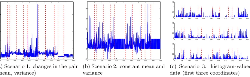
Three scenarios are considered: (1) real-valued data with a changing (mean,variance), (2) real-valued data with constant mean and variance, and (3) histogram-valued data as in Example 4.
In the three scenarios, the sample size isn= 1 000 and the true segmentationτ?is made ofD?= 11 segments, with change-pointsτ1? = 100,τ2?= 130,τ3? = 220,τ4? = 320,τ5? = 370, τ6? = 520, τ7? = 620, τ8? = 740, τ9? = 790, τ10? = 870 (see Figure 1). For each sample, we choose randomly the distribution of the Xi within each segment of τ? as detailed below;
note that we always make sure that the distribution ofXi does change at each τ`?.
For each scenario, we generate N = 500 independent samples, from which we estimate all quantities that are reported in Section 6.3.
Scenario 1: Real-valued data with changing (mean, variance). The distribution of Xi∈Ris randomly picked out from: B(10,0.2) (binomial),N B(3,0.7) (negative-binomial),
H(10,5,2) (hypergeometric),N(2.5,0.25) (Gaussian),γ(0.5,5) (gamma),W(5,2) (Weibull) andPar(1.5,3) (Pareto). Note that the pair (mean, variance) in each segment changes from that of its neighbors. Table B.1 summarizes its values.
0 100 200 300 400 500 600 700 800 900 1000 0
5 10 15 20 25 30
(a) Scenario 1: changes in the pair (mean, variance)
0 100 200 300 400 500 600 700 800 900 1000 −1
0 1 2 3 4
(b) Scenario 2: constant mean and variance
0 100 200 300 400 500 600 700 800 900 1000
0 0.5 1 1.5
0 100 200 300 400 500 600 700 800 900 1000
0 0.5 1 1.5
0 100 200 300 400 500 600 700 800 900 1000
0 0.5 1 1.5
(c) Scenario 3: histogram-valued data (first three coordinates)
Figure 1: Examples of generated signals (blue plain curve) in the three scenarios. Red vertical dashed lines visualize the true change-points locations.
The variables S` are generated as follows: S1 is uniformly chosen among {1, . . . ,7}, and for every ` ∈ {1, . . . , D?−1}, given S`, S`+1 is uniformly chosen among {1, . . . ,7}\{S`}.
Figure 1a shows one sample generated according to this scenario.
Scenario 2: Real-valued data with constant mean and variance. The distribution of Xi ∈R is randomly chosen among (1) B(0.5) (Bernoulli), (2) N(0.5,0.25) (Gaussian) and (3)E(0.5) (exponential). These three distributions have a mean 0.5 and a variance 0.25.
The distribution within segment `∈ {1, . . . , D?}is given by the realization of a random
variableS` ∈ {1,2,3}, similarly to what is done in scenario 1 (replacing 7 by 3). Figure 1b
shows one sample generated according to this scenario.
Scenario 3: Histogram-valued data. The observations Xi belong to the d-dimensional
simplex withd= 20 (Example 4), that is,Xi = (a1, . . . , ad)∈[0,1]d withPdj=1aj = 1. For
each ` ∈ {1, . . . , D?}, we randomly generate d parameter values p`1, . . . , p`d independently with uniform distribution over [0, c3] with c3 = 0.2 . Then, within the `-th segment of τ?, Xi follows a Dirichlet distribution with parameter (p`1, . . . , p`d). Figure 1c displays the first
three coordinates of one sample generated according to this scenario.
6.2. Parameters of KCP
For each sample, we apply the kernel change-point procedure (KCP, that is, Algorithm 1) with the following choices for its parameters. We always take Dmax= 100.
For the first two scenarios, we consider three kernels:
(i) The linear kernel klin(x, y) =xy.
(ii) The Hermite kernel given bykHσH(x, y) defined in Section 3.2. In scenario 1,σH = 1.
In scenario 2,σH = 0.1.
(iii) The Gaussian kernelkσGGdefined in Section 3.2. In scenario 1,σG = 0.1. In scenario 2,
σG= 0.16.
In each scenario several candidate values have been explored for the bandwidth param-eters of the above kernels. We have selected the ones with the most representative results.
For choosing the constants c1, c2 arising from Step 2 of KCP, we use the “slope heuris-tics” method, and more precisely a variant proposed by Lebarbier (2002, Section 4.3.2) for the calibration of two constants for change-point detection. We first perform a linear regression ofRbn(
b
τ(D)) against 1/n·log Dn−−11and D/nforD∈[0.6×Dmax, Dmax]. Then, denoting by bs1,bs2 the coefficients obtained, we define ci = −αbsi for i= 1,2, with α = 2.
The slope heuristics is justified theoretically in various settings (for instance by Arlot and Massart, 2009, for regressograms; see Arlot, 2019, for a survey) and is supported by nu-merous experiments (Baudry et al., 2012), including for change-point detection (Lebarbier, 2002, 2005). A partial theoretical justification has been obtained recently for change-point detection (Sorba, 2017). The intuition behind the slope heuristics is that the minimal amount of penalization needed for avoiding to overfit with bτ ∈ argminτ{Rbn(τ) + pen(τ)}
and the optimal penalty (approximately) are proportional:
penoptimal(τ)≈αpenminimal(τ)
for some constantα >1, equal to 2 in several settings. The linear regression step described above corresponds to estimating the minimal penalty:
penminimal(τ)≈ −sb1· 1 nlog
n−1 Dτ−1
−bs2
Dτ
n ·
Then, multiplying it byαleads to an estimation of the optimal penalty. In the experiments, we considered several values ofα∈[0.8,2.5]. Remarkably, the performance of the procedure is not too sensitive to the value of α providedα∈[1.7,2.2]. We only report the results for α= 2 because it corresponds to the classical advice when using the slope heuristics, and it is among the best choices for α according to the experiments.
6.3. Results
We now summarize the results of the experiments.
6.3.1. Distance Between Segmentations
In order to assess the quality of the segmentationbτ as an estimator of the true segmentation
τ?, we consider two measures of distance between segmentations. For any τ, τ0 ∈ Tn, we
define the Hausdorff distance betweenτ andτ0 by
dH(τ, τ0) := max
max 16i6Dτ−1
min 16j6Dτ0−1
τi−τj0
, max
16j6Dτ0−1
min 16i6Dτ−1
τi−τj0
and the Frobenius distance betweenτ and τ0 (Lajugie et al., 2014) by
dF(τ, τ0) :=
M
τ −Mτ0
F =
s X
16i,j6n
(Mτ i,j−Mτ
0 i,j)2,
0 20 40 60 80 100
0 20 40 60 80 100
Dimension D
Frobenius dist.
0 20 40 60 80 1000
100 200 300 400 500
Hausdorff dist.
Frobenius Hausdorff
(a) Average distance (dFordH) betweenbτ(D) andτ
?
,
as a function ofD
0 20 40 60 80 100
−150 −100 −50 0 50 100 150
Dimension D
Penalized crit Risk Empirical risk
(b) Average risk R bµ
b
τ(D)
, empirical risk
b
Rn(bτ(D)) and penalized criterion as a function
ofD
4 5 6 7 8 9 10 11 12 13 14 15
0 0.05 0.1 0.15 0.2 0.25 0.3 0.35 0.4 0.45 0.5
Dimension D
Frequency of selection
(c) Distribution ofDb
100 200 300 400 500 600 700 800 900 1000
0 0.1 0.2 0.3 0.4 0.5 0.6
Position
Freq. of selected chgpts
(d) Probability, for each instant i ∈ {1, . . . , n},
thatbτ=bτ(Db) puts a change point ati
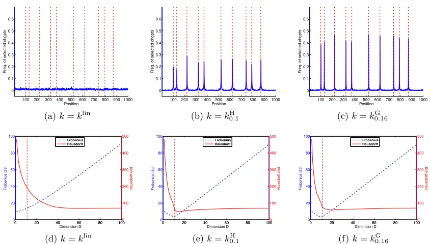
Figure 2: Scenario 1: X =R, variable (mean, variance). Performance of KCP with kernel
k0G.1. The value D? and the localization of the true change points in τ? are materialized by vertical red lines.
Note that Mτ = Πτ the projection matrix onto Fτ when H = R, that is, for the linear kernel onX =R. The Hausdorff distance is probably more classical in the change-point lit-erature, but Figure 2a shows that the Frobenius distance is more informative for comparing (τb(D))D>D?. Indeed, when D is already a bit larger than D?, adding false change points makes the segmentation worse without increasing much dH; on the contrary, d2F readily
6.3.2. Illustration of KCP
Figure 2 illustrates the typical behaviour of KCP whenkis well-suited to the change-point problem we consider. It summarizes results obtained in scenario 1 withk=kGthe Gaussian kernel.
Figure 2a shows the expected distance between the true segmentation τ? and the seg-mentations (τb(D))16D6Dmax produced at Step 1 of KCP. As expected, the distance is clearly minimal at D=D?, for both Hausdorff and Frobenius distances. Note that for each indi-vidual sample, d(τb(D), τ?) behaves exactly as the expectation shown on Figure 2a, up to minor fluctuations. Moreover, the minimal value of the distance is small enough to suggest that bτ(D
?) is indeed close to τ?. For instance,
E[dF(τb(D
?), τ?)]≈1.71, with a 95% error
bar smaller than 0.11. The closeness between bτ(D?) and τ? when k = kG can also be visualized on Figure B.9c in Appendix B.4.
As a comparison, whenk=klin in the same setting,τb(D?) is much further fromτ?since E[dF(bτ(D
?), τ?)]≈10.39±0.24, and a permutation test shows that the difference is
signif-icant, with a p-value smaller than 10−13. See also Figures B.7 and B.9a in Appendix B.4. Step 2 of KCP is illustrated by Figures 2b and 2c. The expectation of the penalized criterion is minimal at D = D? (as well as for the risk of µb
b
τ(D)), and takes significantly larger values whenD6=D? (Figure 2b). As a result, KCP often selects a number of change points Db −1 close to its true value D? −1 (Figure 2c). Overall, this suggests that the
model-selection procedure used at Step 2 of KCP works fairly well.
The overall performance of KCP as a change-point detection procedure is illustrated by Figure 2d. Each true change-point has a probability larger than 0.5 to be recoveredexactly by bτ. If one groups the positionsiby blocks of six elements {6j,6j+ 1, . . . ,6j+ 5},j>1, the frequency of detection of a change point by bτ in each block containing a true change point is between 79 and 89%. Importantly, such figures are obtained without overestimating much the number of change points, according to Figure 2c. Figures B.10a and B.10b in Appendix B.4 show that more standard change-point detection algorithms —that is, KCP withk=klin or kH— have a slightly worse performance.
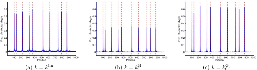
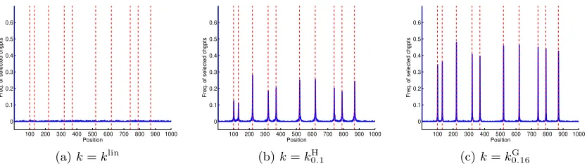
6.3.3. Comparison of Three Kernels in Scenario 2
Scenario 2 proposes a more challenging change-point problem with real-valued data: the distribution of the Xi changes while the mean and the variance remain constant. The
performance of KCP with three kernels —klin,kHand kG— is shown on Figure 3. The lin-ear kernelklincorresponds to the classical least-squares change-point algorithm (Lebarbier, 2005), which is designed to detect changes in the mean, hence it should fail in scenario 2. KCP with the Hermite kernel kH is a natural “hand-made” extension of this classical ap-proach, since it corresponds to applying the least-squares change-point algorithm to the feature vectors (Hj,h(Xi))16j65. By construction, it should be able to detect changes in the first five moments on the Xi. On the contrary, taking k = kG the Gaussian kernel
fully relies on the versatility of KCP, which makes possible to consider (virtually) infinite-dimensional feature vectorskG(Xi,·). SincekG is characteristic, it should be able to detect
any change in the distribution of theXi.
100 200 300 400 500 600 700 800 900 1000 0 0.1 0.2 0.3 0.4 0.5 0.6 Position
Freq. of selected chgpts
(a)k=klin
100 200 300 400 500 600 700 800 900 1000
0 0.1 0.2 0.3 0.4 0.5 0.6 Position
Freq. of selected chgpts
(b)k=kH
0.1
100 200 300 400 500 600 700 800 900 1000
0 0.1 0.2 0.3 0.4 0.5 0.6 Position
Freq. of selected chgpts
(c)k=kG
0.16
0 20 40 60 80 100
0 20 40 60 80 100 Dimension D Frobenius dist.
0 20 40 60 80 1000
100 200 300 400 500 Hausdorff dist. Frobenius Hausdorff
(d)k=klin
0 20 40 60 80 100
0 20 40 60 80 100 Dimension D Frobenius dist.
0 20 40 60 80 1000
100 200 300 400 500 Hausdorff dist. Frobenius Hausdorff
(e)k=kH
0.1
0 20 40 60 80 100
0 20 40 60 80 100 Dimension D Frobenius dist.
0 20 40 60 80 1000
100 200 300 400 500 Hausdorff dist. Frobenius Hausdorff
(f)k=kG
0.16
Figure 3: Scenario 2: X =R, constant mean and variance. Performance of KCP with three different kernels k. The value D? and the localization of the true change points
in τ? are materialized by vertical red lines. Top: Probability, for each instant i∈ {1, . . . , n}, thatτb(D?) puts a change point at i. Bottom: Average distance (dF ordH) betweenτb(D) and τ
?, as a function of D.
number of segments. Then, Figures 3a, 3b and 3c show that klin, kH and kG behave as expected: klinseems to put the change points ofbτ(D?) uniformly at random over{1, . . . , n}, whilekHandkGare able to localize the true change points with a rather large probability of success. The Gaussian kernel here shows a significantly better detection power, compared to kH: the frequency of exact detection of the true change points is between 38 and 47% with kG, and between 17 and 29% with kH. The same holds when considering blocks of size 6: kG then detects the change points with probability 70 to 79%, while kH exhibits probabilities between 58 and 62%.
Figures 3d, 3e and 3f show that a similar comparison between klin, kH, and kG holds over the whole set of segmentations (τb(D))16D6Dmax provided by Step 1 of KCP. With the linear kernel (Figure 3d), the Frobenius distance between τb(D) and τ? is almost minimal forD= 1, which suggests thatτb(D) is not far from random guessing for allD. The shape
of the Hausdorff distance —first decreasing fastly, then almost constant— also supports this interpretation: A small number of purely random guesses do lead to a fast decrease of dH; and for large dimensions, adding a new random guess does not move away τb(D)
from τ? ifτb(D) already contains all the worst possible candidate change points (which are the furthest from the true change points). The Hermite kernel does much better according to Figure 3e: the Frobenius distance from τb(D) to τ
? is minimal for D close to D?, and
the minimal expected distance, infDE[dF(τb(D), τ
much smaller than whenk=klin (in which case infDE[dF(bτ(D), τ
?)]≈10); this difference
is significant (a permutation test yields a p-value smaller than 10−15). Nevertheless, we still obtain slightly better performance for (bτ(D))16D6Dmax withk=k
G, for which the minimal distance to τ? is achieved at D = 9, with a minimal expected value equal to 3.83±0.49 (the difference between kH and kG is not statistically significant). The Hausdorff distance suggests that both kH and kG lead to include false change points among true ones as long asD6D?. However, the smaller Frobenius distance achieved bykG atD= 9 (rather than D= 11 for kH) indicates that the corresponding change points are closer to the true ones than those provided bykH (which include more false positives).
When D= Db is chosen by KCP,kG clearly leads to the best performance in terms of
recovering the exact change points compared toklinandkH, as illustrated by Figures B.11a, B.11b and B.11c in Appendix B.4.
Overall, the best performance for KCP in scenario 2 is clearly obtained with kG, while klin completely fails and kHyields a decent but suboptimal procedure.
We can notice that other settings can lead to different behaviours. For instance, in scenario 1, according to Figure B.10a in Appendix B.4, klin can detect fairly well the true change points —as expected since the mean (almost) always changes in this scenario, see Table B.1 in Appendix B.4—, but this is at the price of a strong overestimation of the number of change points (Figure B.8a). In the same setting,kHprovides fairly good results (Figure B.10b), while kG remains the best choice (Figure 2d).
Since kG is a characteristic kernel, these results suggest that KCP with a characteristic kernel k might be more versatile than classical least-squares change-point algorithms and their extensions. A more detailed simulation experiment would nevertheless be needed to confirm this hypothesis. We also refer to Section 8.2 for a discussion on the choice of kfor a given change-point problem.
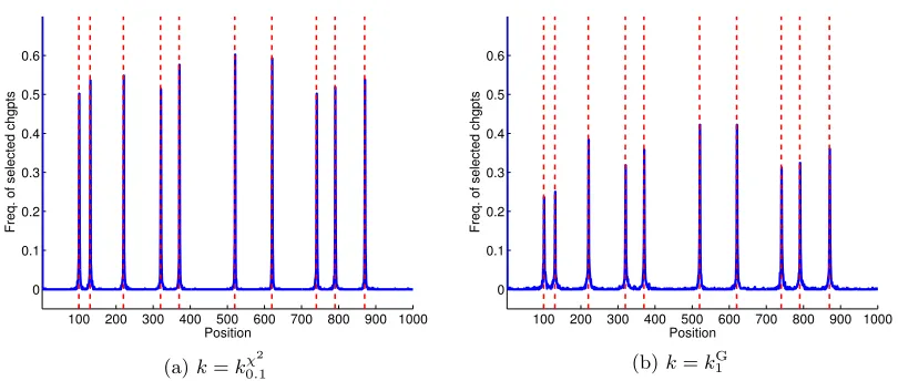
6.3.4. Structured Data
Figure 4 illustrates the performance of KCP on some histogram-valued data (scenario 3). Since a d-dimensional histogram is also an element of Rd, we can analyze such data either with a kernel taking into account the histogram structure (such askχ2) or with a usual kernel onRd(such as klinorkG; here, we considerkG, which seems more reliable according to our experiments in scenarios 1 and 2). Assuming that the number of change points is known, takingk=kχ2 yields quite good results according to Figure 4a, at least in comparison with k=kG (Figure 4b). Similar results hold with a fully data-driven number of change points, as shown by Figures B.13a and B.13b in Appendix B.4. Hence, choosing a kernel such as kχ2, which takes into account the histogram structure of the Xi, can improve much the
change-point detection performance, compared to taking a kernel such askG, which ignores the structure of theXi.