All Models are Wrong, but Many are Useful: Learning a Variable's Importance by Studying an Entire Class of Prediction Models Simultaneously

All Models are Wrong, but

Many

are Useful: Learning a

Variable’s Importance by Studying an Entire Class of

Prediction Models Simultaneously

Aaron Fisher [email protected]

Takeda Pharmaceuticals Cambridge, MA 02139, USA

Cynthia Rudin [email protected]

Departments of Computer Science and Electrical and Computer Engineering Duke University

Durham, NC 27708, USA

Francesca Dominici [email protected]

Department of Biostatistics

Harvard T.H. Chan School of Public Health Boston, MA 02115, USA

(Authors are listed in order of contribution, with highest contribution listed first.)

Editor:Maya Gupta

Abstract

Variable importance (VI) tools describe how much covariates contribute to a prediction model’s accuracy. However, important variables for one well-performing model (for exam-ple, a linear model f(x) =xT_{β with a fixed coefficient vectorβ) may be unimportant for}

another model. In this paper, we propose model class reliance (MCR) as the range of VI values across all well-performing model in a prespecified class. Thus, MCR gives a more comprehensive description of importance by accounting for the fact that many prediction models, possibly of different parametric forms, may fit the data well. In the process of de-riving MCR, we show several informative results for permutation-based VI estimates, based on the VI measures used in Random Forests. Specifically, we derive connections between permutation importance estimates for asingle prediction model, U-statistics, conditional variable importance, conditional causal effects, and linear model coefficients. We then give probabilistic bounds for MCR, using a novel, generalizable technique. We apply MCR to a public data set of Broward County criminal records to study the reliance of recidivism prediction models on sex and race. In this application, MCR can be used to help inform VI for unknown, proprietary models.

Keywords: Rashomon, permutation importance, conditional variable importance, U-statistics, transparency, interpretable models

1. Introduction

Variable importance (VI) tools describe how much a prediction model’s accuracy depends on the information in each covariate. For example, in Random Forests, VI is measured by

c

the decrease in prediction accuracy when a covariate is permuted (Breiman, 2001; Breiman et al., 2001; see also Strobl et al., 2008; Altmann et al., 2010; Zhu et al., 2015; Gregorutti et al., 2015; Datta et al., 2016; Gregorutti et al., 2017). A similar “Perturb” VI measure has been used for neural networks, where noise is added to covariates (Recknagel et al., 1997; Yao et al., 1998; Scardi and Harding, 1999; Gevrey et al., 2003). Such tools can be useful for identifying covariates that must be measured with high precision, for improving the transparency of a “black box” prediction model (see also Rudin, 2019), or for determining what scenarios may cause the model to fail.

However, existing VI measures do not generally account for the fact that many prediction models may fit the data almost equally well. In such cases, the model used by one analyst may rely on entirely different covariate information than the model used by another analyst. This common scenario has been called the “Rashomon” effect of statistics (Breiman et al., 2001; see also Lecu´e, 2011; Statnikov et al., 2013; Tulabandhula and Rudin, 2014; Nevo and Ritov, 2017; Letham et al., 2016). The term is inspired by the 1950 Kurosawa film of the same name, in which four witnesses offer different descriptions and explanations for the same encounter. Under the Rashomon effect, how should analysts give comprehensive descriptions of the importance of each covariate? How well can one analyst recover the conclusions of another? Will the model that gives the best predictions necessarily give the most accurate interpretation?

To address these concerns, we analyze the set of prediction models that provide

near-optimal accuracy, which we refer to as a Rashomon set. This approach stands in contrast

to training to select a single prediction model, among a prespecified class of candidate

models. Our motivation is that Rashomon sets (defined formally below) summarize the range of effective prediction strategies that an analyst might choose. Additionally, even if the candidate models do not contain the true data generating process, we may hope that some of these models function in similar ways to the data generating process. In particular, we may hope there exist well performing candidate models that place the same importance on a variable of interest as the underlying data generating process does. If so, then studying sets of well-performing models will allow us to deduce information about the data generating process.

Applying this approach to study variable importance, we define model class reliance

(MCR) as the highest and lowest degree to which any well-performing model within a given class may rely on a variable of interest for prediction accuracy. Roughly speaking, MCR captures the range of explanations, or mechanisms, associated with well-performing models. Because the resulting range summarizes many prediction models simultaneously, rather a single model, we expect this range to be less affected by the choices that an individual analyst makes during the model-fitting process. Instead of reflecting these choices, MCR aims to reflect the nature of the prediction problem itself.

We make several, specific technical contributions in deriving MCR. First, we review a core measure of how much an individual prediction model relies on covariates of interest

for its accuracy, which we callmodel reliance (MR). This measure is based on permutation

between MR, conditional causal effects, and coefficients for additive models. Expanding

on MR, we propose MCR, which generalizes the definition of MR for a class of models.

We derive finite-sample bounds for MCR, which motivate an intuitive estimator of MCR. Finally, we propose computational procedures for this estimator.

The tools we develop to study Rashomon sets are quite general, and can be used to make finite-sample inferences for arbitrary characteristics of well-performing models. For example, beyond describing variable importance, these tools can describe the range of risk predictions that well-fitting models assign to a particular covariate profile, or the variance of predictions made by well-fitting models. In some cases, these novel techniques may provide finite-sample confidence intervals (CIs) where none have previously existed (see Section 5). MCR and the Rashomon effect become especially relevant in the context of criminal recidivism prediction. Proprietary recidivism risk models trained from criminal records data are increasingly being used in U.S. courtrooms. One concern is that these models may be relying on information that would otherwise be considered unacceptable (for example, race, sex, or proxies for these variables), in order to estimate recidivism risk. The relevant models are often proprietary, and cannot be studied directly. Still, in cases where the predictions made by these models are publicly available, it may be possible to identify alternative prediction models that are sufficiently similar to the proprietary model of interest.

In this paper, we specifically consider the proprietary model COMPAS (Correctional Of-fender Management Profiling for Alternative Sanctions), developed by the company North-pointe Inc. (subsequently, in 2017, NorthNorth-pointe Inc.,Courtview Justice Solutions Inc., and Constellation Justice Systems Inc. joined together under the name Equivant). Our goal is to estimate how much COMPAS relies on either race, sex, or proxies for these variables not measured in our data set. To this end, we apply a broad class of flexible, kernel-based prediction models to predict COMPAS score. In this setting, the MCR interval reflects the highest and lowest degree to which any prediction model in our class can rely on race and sex while still predicting COMPAS score relatively accurately. Equipped with MCR, we can relax the common assumption of being able to correctly specify the unknown model of interest (here, COMPAS) up to a parametric form. Instead, rather than assuming that the COMPAS model itself is contained in our class, we assume that our class contains at least one well-performing alternative model that relies on sensitive covariates to the same degree that COMPAS does. Under this assumption, the MCR interval will contain the VI value for COMPAS. Applying our approach, we find that race, sex, and their potential proxy variables, are likely not the dominant predictive factors in the COMPAS score (see analysis and discussion in Section 10).

MR, causal inference, and conditional variable importance. In Section 9, we illustrate MR and MCR with a simulated toy example, to aid intuition. We also present simulation studies for the task of estimating MR for an unknown, underlying conditional expectation function, under misspecification. We analyze a well-known public data set on recidivism in Section 10, described above. All proofs are presented in the appendices.

2. Notation & Technical Summary

The label of “variable importance” measure has been broadly used to describe approaches for either inference (van der Laan, 2006; D´ıaz et al., 2015; Williamson et al., 2017) or prediction. While these two goals are highly related, we primarily focus on how much prediction models rely on covariates to achieve accuracy. We use terms such as “model reliance” rather than “importance” to clarify this context.

In order to evaluate how much prediction models rely on variables, we now introduce notation for random variables, data, classes of prediction models, and loss functions for

evaluating predictions. LetZ = (Y, X1, X2)∈ Z be a random variable with outcomeY ∈ Y

and covariates X = (X1, X2) ∈ X, where the covariate subsets X1 ∈ X1 and X2 ∈ X2

may each be multivariate. We assume that observations of Z are iid, thatn_≥2, and that

solutions to arg min and arg max operations exist whenever optimizing over sets mentioned in this paper (for example, in Theorem 4, below). Our goal is to study how much different

prediction models rely onX1 to predictY.

We refer to our data set as Z= y X , a matrix composed of a n-length outcome

vectoryin the first column, and an_×pcovariate matrixX= X1 X2

in the remaining

columns. In general, for a given vector v, let v[j] denote its jth element(s). For a given

matrix A, let A0, A[i,·], A[·,j], and A[i,j] respectively denote the transpose of A, the ith

row(s) ofA, the jth _{column(s) ofA, and the element(s) in thei}th_{row(s) and j}th _column(s)

of A.

We use the term model class to refer to a prespecified subset F ⊂ {f | f : X → Y}

of the measurable functions from _X to _Y. We refer to member functions f _{∈ F} as

prediction models, or simply as models. Given a model f, we evaluate its performance

using a nonnegative loss function L : (F × Z) → R≥0. For example, L may be the

squared error loss Lse(f,(y, x1, x2)) = (y −f(x1, x2))2 for regression, or the hinge loss

Lh(f,(y, x1, x2)) = (1−yf(x1, x2))+ for classification. We use the term algorithm to refer

to any procedureA:Zn_{→ F that takes a data set as input and returns a modelf ∈ F as}

output.

2.1. Summary of Rashomon Sets & Model Class Reliance

Many traditional statistical estimates come from descriptions of a single, fitted

predic-tion model. In contrast, in this secpredic-tion, we summarize our approach for studying a set

of near-optimal models. To define this set, we require a prespecified “reference” model,

denoted byfref, to serve as a benchmark for predictive performance. For example,fref may

come from a flowchart used to predict injury severity in a hospital’s emergency room, or from another quantitative decision rule that is currently implemented in practice. Given

with expected loss no more than above that of fref. We denote this set as R() :=

{f ∈ F : EL(f, Z)≤EL(fref, Z) +}, where E denotes expectations with respect to the

population distribution. This set can be thought of as representing models that might be arrived at due to differences in data measurement, processing, filtering, model parameteri-zation, covariate selection, or other analysis choices (see Section 4).

✏ fref

More accurate Less accurate

EL(f, Z)

Rely less onX1

Rely more onX1

M R(f)

M CR+(✏)

M CR (✏)

✏ fref

Rely less onX1

Rely more onX1

\

M CR (✏) M CR+\ (✏)

ˆ

EL(f, Z)

d

M R(f)

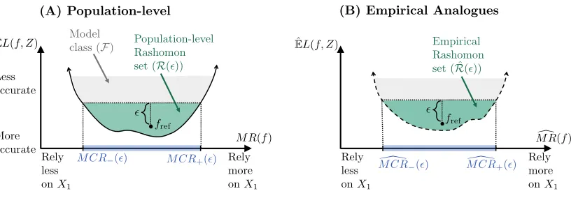
(A) Population-level (B) Empirical Analogues

Illustrations of Rashomon Sets & Model Class Reliance

Model

class (F) Empirical

Rashomon set ( ˆR(✏)) Population-level

Rashomon set (R(✏))

Figure 1: Rashomon sets and model class reliance – Panel (A) illustrates a hypothetical

Rashomon setR(), within a model class F. The y-axis shows the expected loss

of each modelf _{∈ F}, and the x-axis shows how much each modelf relies onX1

(defined formally in Section 3). Along the x-axis, the population-level MCR range is highlighted in blue, showing the values of MR corresponding to well-performing models (see Section 4). Panel (B) shows the in-sample analogue of Panel (A).

Here, the y-axis denotes the in-sample loss, ˆEL(f, Z) := 1

n Pn

i=1L(f,Z[i,·]); the

x-axis shows the empirical model reliance of each modelf ∈ F onX1(see Section

3); and the highlighted portion of the x-axis shows empirical MCR (see Section 4).

Figure 1-A illustrates a hypothetical example of a population -Rashomon set. Here,

the y-axis shows the expected loss of each model f ∈ F, and the x-axis shows how much

each model relies on X1 for its predictive accuracy. More specifically, given a prediction

model f, the x-axis shows the percent increase in f’s expected loss when noise is added to

X1. We refer to this measure as themodel reliance (MR) off onX1, written informally as

M R(f) := Expected loss of f under noise

Expected loss off without noise. (2.1)

The added noise must satisfy certain properties, namely, it must render X1 completely

uninformative of the outcome Y, without altering the marginal distribution of X1 (for

details, see Section 3, as well as Breiman, 2001; Breiman et al., 2001).

Our central goal is to understand how much, or how little, models may rely on covariates

is shown by the highlighted interval along the x-axis. We refer to an interval of this type as a population-level model class reliance (MCR) range (see Section 4), formally defined as

[M CR−(), M CR+()] :=

min

f∈R()M R(f), fmax∈R()M R(f)

. (2.2)

To estimate this range, we use empirical analogues of the population -Rashomon set,

and of MR, based on observed data (Figure 1-B). We define an empirical -Rashomon set

as the set of models within-sample loss no more than above that offref, and denote this

set by ˆR(). Informally, we define the empirical MR of a modelf on X1 as

d

M R(f) := In-sample loss of f under noise

In-sample loss of f without noise, (2.3)

that is, the extent to which f appears to rely on X1 in a given sample (see Section 3 for

details). Finally, we define theempirical model class reliance as the range of empirical MR

values corresponding to models with strong in-sample performance (see Section 4), formally written as

[M CR\−(), M CR\+()] :=

"

min

f∈Rˆ() d

M R(f), max

f∈Rˆ() d

M R(f)

#

. (2.4)

In Figure 1-B, the above range is shown by the highlighted portion of the x-axis. We make several technical contributions in the process of developing MCR.

• Estimation of MR, and population-level MCR: Given f, we show desirable

properties ofM Rd(f) as an estimator ofM R(f), using results for U-statistics (Section

3.1 and Theorem 5). We also derive finite sample bounds for population-level MCR,

some of which require a limit on the complexity of_F in the form of a covering

num-ber. These bounds demonstrate that, under fairly weak conditions, empirical MCR provides a sensible estimate of population-level MCR (see Section 4 for details).

• Computation of empirical MCR: Although empirical MCR is fully determined given a sample, the minimization and maximization in Eq 2.4 require nontrivial com-putations. To address this, we outline a general optimization procedure for MCR (Section 6). We give detailed implementations of this procedure for cases when the

model classF is a set of (regularized) linear regression models, or a set of regression

models in a reproducing kernel Hilbert space (Section 7). The output of our

pro-posed procedure is a closed-form, convex envelope containing_F, which can be used to

approximate empirical MCR for any performance level(see Figure 2 for an

illustra-tion). Still, for complex model classes where standard empirical loss minimization is an open problem (for example, neural networks), computing empirical MCR remains an open problem as well.

• Interpretation of MR in terms of model coefficients, and causal effects:

We show that MR for an additive model can be written as a function of the model’s

coefficients (Proposition 15), and that MR for a binary covariate X1 can be written

• Extensions to conditional importance: We provide an extension of MR that is analogous to the notion of conditional importance (Strobl et al., 2008). This extension

describes how much a model relies on the specific information in X1 that cannot

otherwise be gleaned from X2 (Section 8.2).

• Generalizations for Rashomon sets: Beyond notions of variable importance, we also generalize our finite sample results for MCR to describe arbitrary

characteriza-tions of models in a population -Rashomon set. As we discuss in concurrent work

(Coker et al., 2018), this generalization is analogous to the profile likelihood inter-val, and can, for example, be used to bound the range of risk predictions that well-performing prediction models may assign to a particular set of covariates (Section 5).

We begin in the next section by formally reviewing model reliance.

Rely less onX1

Rely more onX1

ˆ

EL(f, Z)

d

M R(f) More

accurate Less

accurate Model classF

\

M CR (✏) M CR+\ (✏)

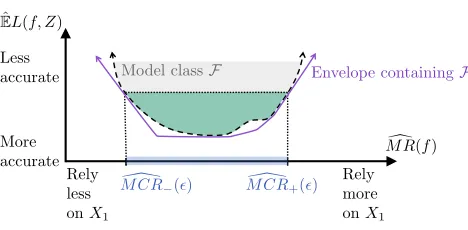
Conservative Computation of Empirical Model Class Reliance

Envelope containingF

Figure 2: Illustration of output from our empirical MCR computational procedure – Our computation procedure produces a closed-form, convex envelope that contains

F (shown above as the solid, purple line), which bounds empirical MCR for any

value of(see Eq 2.4). The procedure works sequentially, tightening these bounds

as much as possible near thevalue of interest (Section 6). The results from our

data analysis (Figure 8) are presented in the same format as the above purple envelope.

3. Model Reliance

To formally describe how much the expected accuracy of a fixed prediction model f relies

on the random variable X1, we use the notion of a “switched” loss where X1 is rendered

uninformative. Throughout this section, we will treatf as a pre-specified prediction model

of interest (as in Hooker, 2007). LetZ(a) _{= (Y}(a)_{, X}(a)

1 , X (a)

2 ) and Z(b) = (Y(b), X

(b) 1 , X

(b) 2 )

be independent random variables, each following the same distribution asZ = (Y, X1, X2).

We define

eswitch(f) :=EL{f,(Y(b), X (a) 1 , X

as representing the expected loss of model f across pairs of observations (Z(a)_{, Z}(b)_{) in}

which the values of X₁(a) and X₁(b) have been switched. To see this interpretation of the

above equation, note that we have used the variables (Y(b)_{, X}(b)

2 ) from Z(b), but we have

used the variable X₁(b) from an independent copy Z(b)_{. This is why we say that X}(a)

1 and

X₁(b) have been switched; the values of (Y(b)_{, X}(a)

1 , X (b)

2 ) do not relate to each other as they

would if they had been chosen together. An alternative interpretation ofeswitch(f) is as the

expected loss of f when noise is added to X1 in such a way that X1 becomes completely

uninformative of Y, but that the marginal distribution of X1 is unchanged.

As a reference point, we compareeswitch(f) against the standard expected loss when none

of the variables are switched,eorig(f) :=EL(f,(Y, X1, X2)). From these two quantities, we

formally define model reliance (MR) as the ratio,

M R(f) := eswitch(f)

eorig(f)

, (3.1)

as we alluded to in Eq 2.1. Higher values ofM R(f) signify greater reliance off onX1. For

example, anM R(f) value of 2 means that the model relies heavily onX1, in the sense that

its loss doubles whenX1 is scrambled. AnM R(f) value of 1 signifies no reliance onX1, in

the sense that the model’s loss does not change whenX1 is scrambled. Models with reliance

values strictly less than 1 are more difficult to interpret, as they rely less on the variable of interest than a random guess. Interestingly, it is possible to have models with reliance

less than one. For instance, a model f0 _{may satisfy M R(f}0_{) <1 if it treats X}

1 and Y as

positively correlated when they are in fact negatively correlated. However, in many cases,

the existence of a model f0 _{∈ F} satisfying M R(f0) < 1 implies the existence of another,

better performing model f00 _{∈ F satisfying M R(f}00_{) = 1 and e}

orig(f00)≤eorig(f0). That is,

although models may exist with MR values less than 1, they will typically be suboptimal (see Appendix A.2).

Model reliance could alternatively be defined as a difference rather than a ratio, that

is, asM Rdifference(f) :=eswitch(f)−eorig(f). In Appendix A.5, we discuss how many of our

results remain similar under either definition.

3.1. Estimating Model Reliance with U-statistics, and Connections to Permutation-based Variable Importance

Given a modelf and data setZ= y X , we estimateM R(f) by separately estimating

the numerator and denominator of Eq 3.1. We estimateeorig(f) with the standard empirical

loss,

ˆ

eorig(f) :=

1

n

n X

i=1

L{f,(y[i],X1[i,·],X2[i,·])}. (3.2)

We estimate eswitch(f) by performing a “switch” operation across all observed pairs, as in

ˆ

eswitch(f) :=

1

n(n−1)

n X

i=1 X

j6=i

L_{f,(y_[j],X_1[i,·],X2[j,·])}. (3.3)

Above, we have aggregated over all possible combinations of the observed values for

the summation over all possible pairs (Eq 3.3) is computationally prohibitive due to sample

size, another estimator ofeswitch(f) is

ˆ

edivide(f) : =

1

2bn/2c

bn/2c

X

i=1

L{f,(y[i],X1[i+bn/2c,·],X2[i,·])} (3.4)

+L_{f,(y[i+bn/2c],X1[i,·],X2[i+bn/2c,·])}

. (3.5)

Here, rather than summing over all pairs, we divide the sample in half. We then match the

first half’s values for (Y, X2) with the second half’s values forX1 (Line 3.4), and vice versa

(Line 3.5). All three of the above estimators (Eqs 3.2, 3.3 & 3.5) are unbiased for their respective estimands, as we discuss in more detail shortly.

Finally, we can estimate M R(f) with the plug-in estimator

d

M R(f) := eˆswitch(f) ˆ

eorig(f)

, (3.6)

which we define as the empirical model reliance of f on X1. In this way, we formalize the

empirical MR definition in Eq 2.3.

Again, our definition of empirical MR is very similar to the permutation-based vari-able importance approach of Breiman (2001), where Breiman uses a single random per-mutation and we consider all possible pairs. To compare these two approaches more

pre-cisely, let _{π1, . . . ,πn!} be a set of n-length vectors, each containing a different

permu-tation of the set {1, . . . , n}. The approach of Breiman (2001) is analogous to

comput-ing the loss Pn_i=1L_{f,(y[i],X1[πl[i],·],X2[i,·])} for a randomly chosen permutation vector

πl∈ {π1, . . . ,πn!}. Similarly, our calculation in Eq 3.3 is proportional to the sum of losses

over all possible (n!) permutations, excluding the n unique combinations of the rows of

X1 and the rows of

X2 y

that appear in the original sample (see Appendix A.3). Excluding these observations is necessary to preserve the (finite-sample) unbiasedness of ˆ

eswitch(f).

The estimators ˆeorig(f), ˆeswitch(f) and ˆedivide(f) all belong to the well-studied class of

U-statistics. Thus, under fairly minor conditions, these estimators are unbiased, asymptot-ically normal, and have finite-sample probabilistic bounds (Hoeffding, 1948, 1963; Serfling, 1980; see also DeLong et al., 1988 for an early use of U-statistics in machine learning, as well as caveats in Demler et al., 2012). To our knowledge, connections between permutation-based importance and U-statistics have not been previously established.

While the above results from U-statistics depend on the model f being fixed a priori,

we can also leverage these results to create uniform bounds on the MR estimation error

for all models in a sufficiently regularized class _F. We formally present this bound in

Section 4 (Theorem 5), after introducing required conditions on model class complexity. The existence of this uniform bound implies that it is feasible to train a model and to

evaluate its importance using the same data. This differs from the classical VI approach of

Random Forests (Breiman, 2001), which avoids in-sample importance estimation. There, each tree in the ensemble is fit on a random subset of data, and VI for the tree is estimated using the held-out data. The tree-specific VI estimates are then aggregated to obtain a VI estimate for the overall ensemble. Although sample-splitting approaches such as this are helpful in many cases, the uniform bound for MR suggests that they are not strictly

3.2. Limitations of Existing Variable Importance Methods

Several common approaches for variable selection, or for describing relationships between variables, do not necessarily capture a variable’s importance. Null hypothesis testing meth-ods may identify a relationship, but do not describe the relationship’s strength. Similarly, checking whether a variable is included by a sparse model-fitting algorithm, such as the Lasso (Hastie et al., 2009), does not describe the extent to which the variable is relied on. Partial dependence plots (Breiman et al., 2001; Hastie et al., 2009) can be difficult to in-terpret if multiple variables are of interest, or if the prediction model contains interaction effects.

Another common VI procedure is to run a model-fitting algorithm twice, first on all

of the data, and then again after removing X1 from the data set. The losses for the two

resulting models are then compared to determine the importance, or “necessity,” of X1

(Gevrey et al., 2003). Because this measure is a function of two prediction models rather

than one, it does not measure how much either individual model relies on X1. We refer

to this approach as measuring empirical Algorithm Reliance (AR) on X1, as the

model-fitting algorithm is the common attribute between the two models. Related procedures were proposed by Breiman et al. (2001); Breiman (2001), which measure the sufficiency of

X1.

As we discuss in Section 3.1, the permutation-based VI measure from RFs (Breiman, 2001; Breiman et al., 2001) forms the inspiration for our definition of MR. This RF VI measure has been the topic of empirical studies (Archer and Kimes, 2008; Calle and Urrea, 2010; Wang et al., 2016), and several variations of the measure have been proposed (Strobl et al., 2007, 2008; Altmann et al., 2010; Hapfelmeier et al., 2014). Mentch and Hooker (2016) use U-statistics to study predictions of ensemble models fit to subsamples, similar to the bootstrap aggregation used in RFs. Procedures related to “Mean Difference Impurity,” another VI measure derived for RFs, have been studied theoretically by Louppe et al. (2013); Kazemitabar et al. (2017). All of this literature focuses on VI measures for RFs, for ensembles, or for individual trees. Our estimator for model reliance differs from the traditional RF VI measure (Breiman, 2001) in that we permute inputs to the overall model, rather than permuting the inputs to each individual ensemble member. Thus, our approach can be used generally, and is not limited to trees or ensemble models.

Outside of the context of RF VI, Zhu et al. (2015) propose an estimand similar to our definition of model reliance, and Gregorutti et al. (2015, 2017) propose an estimand

analogous to eswitch(f)−eorig(f). These recent works focus on the model reliance of f

on X1 specifically when f is equal to the conditional expectation function of Y (that is,

f(x1, x2) = E[Y|X1 =x1, X2 =x2]). In contrast, we consider model reliance for arbitrary

prediction models f. Datta et al. (2016) study the extent to which a model’s predictions

are expected to change when a subset of variables is permuted, regardless of whether the

permutation affects a loss functionL. These VI approaches are specific to a single prediction

model, as is MR. In the next section, we consider a more general conception of importance:

4. Model Class Reliance

Like many statistical procedures, our MR measure (Section 3) produces a description of a

single predictive model. Given a model with high predictive accuracy, MR describes how

much the model’s performance hinges on covariates of interest (X1). However, there will

often be many other models that perform similarly well, and that rely on X1 to different

degrees. With this notion in mind, we now study how much any well-performing model

from a prespecified class_F may rely on covariates of interest.

Recall from Section 2.1 that, in order to define a population -Rashomon set of

near-optimal models, we must choose a “reference” model fref to serve as a performance

bench-mark. In order to discuss this choice, we now introduce more explicit notation for the

population-Rashomon set, written as

R(, fref,F) :={f ∈ F : eorig(f)≤eorig(fref) +}. (4.1)

Note that we write _R(, fref,F) and R() interchangeably whenfref and F are clear from

context. Similarly, we occasionally write empirical-Rashomon sets using the more explicit

notation ˆR(, fref,F) :={f ∈ F : ˆeorig(f)≤eˆorig(fref) +}, but typically abbreviate these

sets as ˆ_R().

While fref could be selected by minimizing the in-sample loss, the theoretical study of

R(, fref,F) is simplified under the assumption that fref is prespecified. For example, fref

may come from a flowchart used to predict injury severity in a hospital’s emergency room, or from another quantitative decision rule that is currently implemented in practice. The

model fref can also be selected using sample splitting. In some cases it may be desirable

to fix fref equal to the best-in-class model f? := arg minf∈Feorig(f), but this is generally

infeasible because f? _{is unknown. Still, for any f}

ref ∈ F, the Rashomon set R(, fref,F)

defined using fref will always be conservative in the sense that it contains the Rashomon

set R(, f?_{,F) defined usingf}?_.

We can now formalize our definitions of population-level MCR and empirical MCR by

simply plugging in our definitions for M R(f) and M Rd(f) (Section 3) into Eqs 2.2 & 2.4

respectively. Studying population-level MCR (Eq 2.2) is the main focus of this paper, as it provides a more comprehensive view of importance than measures from a single model. If

M CR+() is low, thenno well-performing model inF places high importance on X1, and

X1 can be discarded at low cost regardless of future modeling decisions. If M CR−() is

large, thenevery well-performing model in_F must rely substantially onX1, andX1 should

be given careful attention during the modeling process. Here,_F may itself consist of several

parametric model forms (for example, all linear models and all decision tree models with

less than 6 single-split nodes). We stress that the range [M CR−(), M CR+()] does not

depend on the fitting algorithm used to select a model f _{∈ F}. The range is valid for any

algorithm producing models in F, and applies for anyf ∈ F.

In the remainder of this section, we derive finite sample bounds for population-level MCR, from which we argue that empirical MCR provides reasonable estimates of population-level MCR (Section 4.1). In Appendix B.7 we consider an alternate formulation of Rashomon

sets and MCR where we replace the relative loss threshold in the definition of _R() with

an absolute loss threshold. This alternate formulation can be similar in practice, but still

requires the specification of a reference function fref to ensure that R() and ˆR() are

4.1. Motivating Empirical Estimators of MCR by Deriving Finite-sample Bounds

In this section we derive finite-sample, probabilistic bounds for M CR+() and M CR−().

Our results imply that, under minimal assumptions, M CR\+() and M CR\−() are

respec-tively within a neighborhood ofM CR+() and M CR−() with high probability. However,

the weakness of our assumptions (which are typical for statistical-learning-theoretic anal-ysis) renders the width of our resulting CIs to be impractically large, and so we use these

results only to show conditions under which M CR\+() and M CR\−() form sensible point

estimates. In Sections 9.1 & 10, below, we apply a bootstrap procedure to account for sampling variability.

To derive these results we introduce three bounded loss assumptions, each of which can

be assessed empirically. Let borig, Bind, Bref, Bswitch ∈Rbe known constants.

Assumption 1 (Bounded individual loss) For a given model f ∈ F, assume that 0 ≤

L(f,(y, x1, x2))≤Bind for any (y, x1, x2)∈(Y × X1× X2).

Assumption 2 (Bounded relative loss) For a given modelf _{∈ F}, assume that_|L(f,(y, x1, x2))−

L(fref,(y, x1, x2))| ≤Bref for any (y, x1, x2)∈ Z.

Assumption 3 (Bounded aggregate loss) For a given model f _{∈ F}, assume that P_{0 < borig≤eˆorig(f)}=P{eˆswitch(f)≤Bswitch}= 1.

Each assumption is a property of a specific model f _{∈ F}. The notation Bind and Bref

refer to bounds for any individual observation, and the notation borig and Bswitch refer to

bounds on the aggregated loss L in a sample. These boundedness assumptions are central

to our finite sample guarantees, shown below.

Crucially, loss functions L that are unbounded in general may be used so long as

L(f,(y, x1, x2)) is bounded on a particular domain. For example, the squared-error loss

can be used ifY is contained within a known range, and predictionsf(x1, x2) are contained

within the same range for (x1, x2) ∈ X × X2. We give example methods of determining

Bind in Sections 7.3.2 & 7.4.2. For Assumption 3, we can approximate borig by training a

highly flexible model to the data, and setting borig equal to half (or any positive fraction)

of the resulting cross-validated loss. To determineBswitch we can simply setBswitch=Bind,

although this may be conservative. For example, in the case of binary classification models for non-separable groups (see Section 9.1), no linear classifier can misclassify all

observa-tions, particularly after a covariate is permuted. Thus, it must hold that Bind > Bswitch.

Similarly, if fref satisfies Assumption 1, thenBref may be conservatively set equal to Bind.

If model reliance is redefined as a difference rather than a ratio, then a similar form of the results in this section will apply without Assumption 3 (see Appendix A.5).

Based on these assumptions, we can create a finite-sample upper bound for M CR+()

and lower bound forM CR−(). In other words, we create an “outer” bound that contains

the interval [M CR−(), M CR+()] with high probability.

Theorem 4 (“Outer” MCR Bounds) Given a constant≥0, letf+,∈arg maxR()M R(f)

reliance among models in _R(). If f+, and f−, satisfy Assumptions 1, 2 & 3, then PM CR+()>M CR\+(out) +Qout

≤δ, and (4.2)

PM CR−()<M CR\−(out)− Qout

≤δ, (4.3)

where out:=+ 2Bref

q

log(3δ−1₎

2n , and Qout:= Bswitch

borig −

Bswitch−Bind q

log(6δ−1)

n

borig+Bind q

log(6δ−1) 2n

.

Eq 4.2 states that, with high probability, M CR+() is no higher than M CR\+(out)

added to an error term _Qout. As nincreases, out approaches and Qout approaches zero.

One practical implication is that, roughly speaking, if M CR\+()≈M CR\+(out), then the

empirical estimator M CR\+() is unlikely to substantially underestimate M CR+(). By

similar reasoning, we can conclude from Eq 4.3 that if M CR\−() ≈ M CR\−(out), then

\

M CR−() is unlikely to substantially overestimateM CR−(). By setting= 0, Theorem

4 can also be used to create a finite-sample bound for the reliance of the unique (unknown)

best-in-class model onX1(see Corollary 22 in Appendix A.4), although describing individual

models is not the main focus of this paper.

We provide a visual illustration of Theorem 4 in Figure 3. A brief sketch of the proof

is as follows. First, we enlarge the empirical -Rashomon set by increasing to out, such

that, by Hoeffding’s inequality,f+,∈Rˆ(out) with high probability. Whenf+, ∈Rˆ(out),

we know that M Rd(f+,) ≤ M CR\+(out) by the definition of M CR\+(out). Next, the

term_Qout leverages finite-sample results for U-statistics to account for estimation error of

M R(f+,) =M CR+() when using the estimatorM Rd(f+,). Thus, we can relateM Rd(f+,)

to bothM CR\+(out) andM CR+() in order to obtain Eq 4.2. Similar steps can be applied

to obtain Eq 4.3.

The bounds in Theorem 4 naturally account for potential overfitting without an explicit limit on model class complexity (such as a covering number, Rademacher complexity, or VC dimension). Instead, these bounds depend on being able to fully optimize MR across

sets in the form of ˆR(). If we allow our model classF to become more flexible, then the

size of ˆ_R() will also increase. Because the bounds in Theorem 4 result from optimizing

over ˆ_R(), increasing the size of ˆ_R() results in wider, more conservative bounds. In this

way, Eqs 4.2 and 4.3 implicitly capture model class complexity.

So far, Theorem 4 lets us bound the range of MR values corresponding to models that predict well, but it does not tell us whether these bounds are actually attained. Similarly,

we can conclude from Theorem 4 that [M CR−(), M CR+()] is unlikely to exceed the

estimated range [M CR\−(),M CR\+()] by a substantial margin, but we cannot determine

whether this estimated range is unnecessarily wide. For example, consider the models

that drive the M CR\+() estimator: the models with strong in-sample accuracy, and high

empirical reliance on X1. These models’ in-sample performance could merely be the result

of overfitting, in which case they do not tell us direct information aboutR(). Alternatively,

even if all of these models truly do perform well on expectation (that is, even if they are

contained in _R()), the model with the highest empirical reliance on X1 may merely be

the model for which our empirical MR estimate contains the most error. Either of these

Fortunately, both problematic scenarios are solved by requiring a limit on the complexity

ofF. We propose a complexity measure in the form of a covering number, which allows us

control a worst case scenario of either overfitting or MR estimation error. Specifically, we

define the set of functions _Gr as an r-margin-expectation-cover if for any f ∈ F and any

distributionD, there existsg∈ Gr such that

EZ∼D|L(f, Z)−L(g, Z)| ≤r. (4.4)

We define thecovering number _N(_F, r) to be the size of the smallestr

-margin-expectation-cover for F. In general, we usePV∼D and EV∼D to denote probabilities and expectations

with respect to a random variable V following the distribution D. We abbreviate these

quantities accordingly when V or D are clear from context, for example, as _PD, PV, or

simplyP. Unless otherwise stated, all expectations and probabilities are taken with respect

to the (unknown) population distribution.

We first show that this complexity measure allows us to control the worst case MR

estimation error, that is, the covering number _N(_F, r) provides a uniform bound on the

error of M Rd(f) for all f _{∈ F}.

Theorem 5 (Uniform bound for M Rd) Given r > 0, if Assumptions 1 and 3 hold for all

f _{∈ F}, then

P "

sup

f∈F

dM R(f)₋M R(f)> q(δ, r, n)

#

≤δ,

where

q(δ, r, n) := Bswitch

borig −

Bswitch−

Bind

q

log(4δ−1_N(F,r√₂₎₎ n + 2r

√

2

borig+

Bind

q

log(4δ−1_N(F,r)) 2n + 2r

. (4.5)

Theorem 5 states that, with high probability, the largest possible estimation error for

M R(f) across all models in_F is bounded byq(δ, r, n), which can be made arbitrarily small

by increasing nand decreasingr. As we noted in Section 3.1, this means that it is possible

to train a model and estimate its reliance on variables without using sample-splitting.

The covering number N(F, r) can also be used to limit the extent of overfitting (see

Appendix B.5.1). As a result, it is possible to set an in-sample performance threshold low enough so that it will only be met by models with strong expected performance (that is, by

models truly within R()). To implement this idea of a stricter performance threshold, we

contract the empirical -Rashomon set by subtracting a buffer term from . This requires

that we generalize the definition of an empirical-Rashomon set to ˆ_R(, fref,F) :={fref} ∪

{f ∈ F : ˆeorig(f)≤eˆorig(fref) +}for∈R, where the explicit inclusion offref now ensures

that ˆR(, fref,F) is nonempty, even for <0. As before, we typically omit the notationfref

and _F, writing ˆ_R() instead.

We are now prepared to answer the questions of whether the bounds from Theorem 4

are actually attained, and of whether the estimated range [M CR\−(),M CR\+()] is

unnec-essarily wide. Our answer comes in the form of an upper bound onM CR−(), and a lower

Theorem 6 (“Inner” MCR Bounds) Given constants_≥0 and r >0, if Assumptions 1, 2 and 3 hold for all f ∈ F, and then

PM CR+()<M CR\+(in)− Qin

≤δ, and (4.6)

PM CR−()>M CR\−(in) +Qin

≤δ, (4.7)

where in :=−2Bref

q

log(4δ−1_N(F,r))

2n −2r, andQin=q δ 2, r, n

, as defined in Eq 4.5.

Theorem 6 can allow us to infer an “inner” bound that is contained within the

in-terval [M CR−(), M CR+()] with high probability. In Figure 3, we illustrate the result

of Theorem 6, and give a sketch of the proof. This proof follows a similar structure to that of Theorem 4, but incorporates Theorem 5’s uniform bound on MR estimation error

(_Qin term), as well as an additional uniform bound on the probability that any model has

in-sample loss too far from its expected loss (in term).

A practical implication of Theorem 6 is that, roughly speaking, ifM CR\+(in)≈M CR\+(),

then it is unlikely for the empirical estimator M CR\+() to substantially underestimate

M CR+(). Taken together with Theorem 4, we can conclude that, if M CR\+(in) ≈

\

M CR+(out), then the estimator M CR\+() is unlikely either to overestimate or to

un-derestimate M CR+() by very much. In large samples, it may be plausible to expect the

condition M CR\+(in) ≈M CR\+(out) to hold, since in and out both approach as n

in-creases. In the same way, if M CR\−(in) ≈M CR\−(out), we can conclude from Eqs 4.3 &

4.7 that the empirical estimator M CR\−() is unlikely to either overestimate or

underesti-mate M CR−() by very much. For this reason, we argue that M CR\−() and M CR\+()

form sensible estimates of population-level MCR – each is contained within a neighborhood of its respective estimand, with high probability. The secondary x-axis of Figure 3 gives an illustration of this argument.

5. Extensions of Rashomon Sets Beyond Variable Importance

In this section we generalize the Rashomon set approach beyond the study of MR. In Section 5.1, we create finite-sample CIs for other summary characterizations of near-optimal, or best-in-class models. The generalization also helps to illustrate a core aspect of the argument underlying Theorem 4: models with near-optimal performance in the population tend to have relatively good performance in random samples.

In Section 5.2, we review existing literature on near-optimal models.

5.1. Finite-sample Confidence Intervals from Rashomon Sets

Rather than describing how much a model relies on X1, here we assume the analyst is

interested in an arbitrary characteristic of a model. We denote this characteristic of interest

asφ:_{F →R}. For example, if fβ is the linear model fβ(x) =x0β, then φ may be defined

as the norm of the associated coefficient vector (that is,φ(fβ) =kβk2

2) or the prediction fβ

!"

# (%)

'

− '

!

,"

-.

'

*

'

!

,"

-/

'

!

,"

-.

'

' − '

!

,"

-.

'

!

,"

-/

'

2̂

05

(%

)

!

,"

-/

'

*

!"

# (%)

!,"

-

'

!,"

-

'

%

Q<latexit sha1_base64="OjtRUuPCOwhZUAEo7uox51HF/uw=">AAACAHicdVDJSgNBFOxxjXEb9eDBS2MQchpmspjMLeDFYwJmgSSEnk4nadKz0P1GDMNc/BUvHhTx6md482/sLIKKFjQUVe/Rr8qLBFdg2x/G2vrG5tZ2Zie7u7d/cGgeHbdUGEvKmjQUoex4RDHBA9YEDoJ1IsmI7wnW9qZXc799y6TiYXADs4j1fTIO+IhTAloamKc9n8CEEpE00kHSA3YHCQ/SdGDmbKtYrlSdS2xbtuuWqkVNymXXdW3sWPYCObRCfWC+94YhjX0WABVEqa5jR9BPiAROBUuzvVixiNApGbOupgHxmeoniwApvtDKEI9CqV8AeKF+30iIr9TM9/Tk/Fz125uLf3ndGEbVvg4UxcACuvxoFAsMIZ63gYdcMgpipgmhkutbMZ0QSSjozrK6hK+k+H/SKlhO0So0SrlaflVHBp2hc5RHDqqgGrpGddREFKXoAT2hZ+PeeDRejNfl6Jqx2jlBP2C8fQKZspel</latexit> in Q<latexit sha1_base64="OjtRUuPCOwhZUAEo7uox51HF/uw=">AAACAHicdVDJSgNBFOxxjXEb9eDBS2MQchpmspjMLeDFYwJmgSSEnk4nadKz0P1GDMNc/BUvHhTx6md482/sLIKKFjQUVe/Rr8qLBFdg2x/G2vrG5tZ2Zie7u7d/cGgeHbdUGEvKmjQUoex4RDHBA9YEDoJ1IsmI7wnW9qZXc799y6TiYXADs4j1fTIO+IhTAloamKc9n8CEEpE00kHSA3YHCQ/SdGDmbKtYrlSdS2xbtuuWqkVNymXXdW3sWPYCObRCfWC+94YhjX0WABVEqa5jR9BPiAROBUuzvVixiNApGbOupgHxmeoniwApvtDKEI9CqV8AeKF+30iIr9TM9/Tk/Fz125uLf3ndGEbVvg4UxcACuvxoFAsMIZ63gYdcMgpipgmhkutbMZ0QSSjozrK6hK+k+H/SKlhO0So0SrlaflVHBp2hc5RHDqqgGrpGddREFKXoAT2hZ+PeeDRejNfl6Jqx2jlBP2C8fQKZspel</latexit> in

Qout<latexit sha1_base64="I6/HDX4jYugG0z4q2yu26oC1pLw=">AAACAXicdVDJSgNBEO1xjXGLehG8NAYhp2EmMzHxFvDiMQGzQBJCT6eTNOlZ6K4RwzBe/BUvHhTx6l9482/sLIKKPih4vFdFVT0vElyBZX0YK6tr6xubma3s9s7u3n7u4LCpwlhS1qChCGXbI4oJHrAGcBCsHUlGfE+wlje5nPmtGyYVD4NrmEas55NRwIecEtBSP3fc9QmMKRFJPe0nXWC3kIQxpGk/l7fMolMqWRVsma7ruO6FJuXSecl2sG1ac+TRErV+7r07CGnsswCoIEp1bCuCXkIkcCpYmu3GikWETsiIdTQNiM9UL5l/kOIzrQzwMJS6AsBz9ftEQnylpr6nO2f3qt/eTPzL68QwrPQSHkQxsIAuFg1jgSHEszjwgEtGQUw1IVRyfSumYyIJBR1aVofw9Sn+nzSLpu2YxbqbrxaWcWTQCTpFBWSjMqqiK1RDDUTRHXpAT+jZuDcejRfjddG6YixnjtAPGG+fbJGYGg==</latexit> Qout

<latexit sha1_base64="I6/HDX4jYugG0z4q2yu26oC1pLw=">AAACAXicdVDJSgNBEO1xjXGLehG8NAYhp2EmMzHxFvDiMQGzQBJCT6eTNOlZ6K4RwzBe/BUvHhTx6l9482/sLIKKPih4vFdFVT0vElyBZX0YK6tr6xubma3s9s7u3n7u4LCpwlhS1qChCGXbI4oJHrAGcBCsHUlGfE+wlje5nPmtGyYVD4NrmEas55NRwIecEtBSP3fc9QmMKRFJPe0nXWC3kIQxpGk/l7fMolMqWRVsma7ruO6FJuXSecl2sG1ac+TRErV+7r07CGnsswCoIEp1bCuCXkIkcCpYmu3GikWETsiIdTQNiM9UL5l/kOIzrQzwMJS6AsBz9ftEQnylpr6nO2f3qt/eTPzL68QwrPQSHkQxsIAuFg1jgSHEszjwgEtGQUw1IVRyfSumYyIJBR1aVofw9Sn+nzSLpu2YxbqbrxaWcWTQCTpFBWSjMqqiK1RDDUTRHXpAT+jZuDcejRfjddG6YixnjtAPGG+fbJGYGg==</latexit>

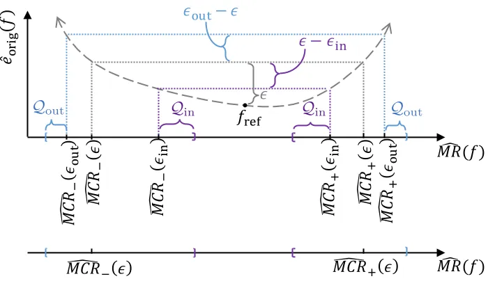
Figure 3: Illustration of terms in Theorems 4 and 6 – Above we show the relation between

empirical MR (x-axis) and empirical loss (y-axis) for modelsf in a hypothetical

model classF. We markfref by the black point. For each possible model reliance

valuer _≥0, the curved, dashed line shows the lowest possible empirical loss for

a function in f _{∈ F} satisfying M Rd(f) = r. The set ˆ_R() contains all models

in F within the dotted gray lines. To create the bounds from Theorem 4, we

expand the empirical-Rashomon set by increasing toout, such that f+, (or

f−,) is contained in ˆR(out) with high probability. We then add (or subtract)

Qout to account for estimation error of M Rd(f+,) (or M Rd(f−,)). These steps

are illustrated above in blue, with the final bounds shown by the blue bracket

symbols along the x-axis. To create the bounds forM CR+() (andM CR−()) in

Theorem 6, we constrict the empirical-Rashomon set by decreasingtoin, such

that all models with high expected loss are simultaneously excluded from ˆ_R(in)

with high probability. We then subtract (or add)Qin to simultaneously account

for MR estimation error for models in ˆ_R(in). These steps are illustrated above

in purple, with the final bounds shown by the purple bracket symbols along the x-axis. For emphasis, below this figure we show a copy of the x-axis with

selected annotations, from which it is clear that M CR\−() and M CR\+() are

always within the bounds produced by Theorems 4 and 6. With high probability,

\

M CR−() andM CR\+() are within a neighborhood ofM CR−() andM CR+()

Given a descriptor φ, we now show a general result that allows creation of finite-sample

CIs for the best performing models R(). The resulting CIs are themselves based on

em-pirical Rashomon sets.

Proposition 7 (Finite sample CIs from Rashomon sets) Let 0 :=+ 2Bref

q

log(2δ−1₎ 2n , let

ˆ

φ−(0) := min_f∈Rˆ(0₎φ(f) and let φˆ+(0) := max_f∈Rˆ(0₎φ(f).

If Assumption 2 holds for all f ∈ R(), then

Ph{φ(f) :f ∈ R()} ⊆hφˆ−(0),φˆ+(0) ii

≥1−δ.

Proposition 7 generates a finite-sample CI for the range of values φ(f) corresponding to

well-performing models, {φ(f) :f ∈ R()}. This CI, denoted byhφˆ−(0),φˆ+(0)

i

, can itself

be interpreted as the range of valuesφ(f) corresponding to modelsf with empirical loss not

substantially above that of fref. Thus, the interval has both a rigorous coverage rate and

a coherent in-sample interpretation. The proof of Proposition 7 uses Hoeffding’s inequality

to show that models in_F are contained in ˆ_R(0) with high probability, that is, that models

with good expected performance tend to perform well in random samples.

An immediate corollary of Proposition 7 is that we can generate finite-sample CIs for

all best-in-class models f? _{∈arg min}

f∈FEL(f, Z) by setting = 0. This corollary can be

further strengthened if a single model f? _{is assumed to uniquely minimize EL(f, Z) over}

f ∈ F (see Appendix B.6).

Note that Proposition 7 implicitly assumes thatφ(f) can be determined exactly for any

model f _{∈ F}, in order for the interval hφˆ−(0),φˆ+(0)

i

to be precisely determined. This

assumption does not hold, for example, if φ(f) = M R(f), or if φ(f) = Var{f(X1, X2)},

as these quantities depend on both f and the (unknown) population distribution. In such

cases, an additional correction factor must be incorporated to account for estimation error

of φ(f), such as theQout term in Theorem 4.

In concurrent work, Coker et al. (2018) show that profile likelihood intervals take the

same form as the interval [ ˆφ−(0),φˆ+(0)] in Proposition 7. This means that a profile

like-lihood interval can also be expressed by minimizing and maximizing over an empirical

Rashomon set. More specifically, consider the case where the loss functionLis the negative

of theknown log likelihood function, and wherefref is the maximum likelihood estimate of

the “true model,” which in this case is f?_{. If additional minor assumptions are met (see}

Appendix A.6 for details), then the (1₋δ)-level profile likelihood interval forφ(f?_{) is equal}

to [ ˆφ−(χ1_2n,1−δ),φˆ+(

χ1,1−δ

2n )], where ˆφ− and ˆφ+ are defined as in Proposition 7, andχ1,1−δ is

the 1−δ percentile of a chi-square distribution with 1 degree of freedom.

Relative to a profile likelihood approach, the advantage of Proposition 7 is that it does not require asymptotics, it does not require that the likelihood be known up to a parametric

form, and it can be extended to study thesetof near-optimal prediction modelsR(), rather

than a single, potentially misspecified prediction model f?_{. This is especially useful when}

different near-optimal models accurately describe different aspects of the underlying data generating process, but none capture it completely. The disadvantage of Proposition 7 is

that the required performance threshold of 0 _{=+ 2B}

ref q

log(2δ−1₎

2n decreases more slowly

than the performance threshold of χ1,1−δ

our results from Section 4.1 carry a similar disadvantage, we use these results primarily to

motivate point estimates describing the Rashomon set R().

Still, it is worth emphasizing the generality of Proposition 7. Through this result, Rashomon sets allow us to reframe a wide set of finite-sample inference problems as in-sample optimization problems. The implied CIs are not necessarily in closed form, but the approach still opens an exciting pathway for deriving non-asymptotic results. For example, they imply that existing methods for profile likelihood intervals might be able to be reapplied to achieve finite-sample results. For highly complex model classes where profile likelihoods are difficult to compute, such as neural networks or random forests, approximate inference is sometimes achieved via approximate optimization procedures (for example, Markov chain Monte Carlo for Bayesian additive regression trees, in Chipman et al., 2010). Proposition

7 shows that similar approximate optimization methods could be repurposed to establish

approximate, finite-sample inferences for the same model classes.

5.2. Related Literature on the Rashomon Effect

Breiman et al. (2001) introduced the “Rashomon effect” of statistics as a problem of ambi-guity: if many models fit the data well, it is unclear which model we should try to interpret. Breiman suggests that the ensembling many well-performing models together can resolve this ambiguity, as the new ensemble model may perform better than any of its individual members. However, this approach may only push the problem from the member level to the ensemble level, as there may also be many different ensemble models that fit the data well.

The Rashomon effect has also been considered in several subject areas outside of VI, in-cluding those in non-statistical academic disciplines (Heider, 1988; Roth and Mehta, 2002). Tulabandhula and Rudin (2014) optimize a decision rule to perform well under the pre-dicted range of outcomes from any well-performing model. Statnikov et al. (2013) propose an algorithm to discover multiple Markov boundaries, that is, minimal sets of covariates such that conditioning on any one set induces independence between the outcome and the remaining covariates. Nevo and Ritov (2017) report interpretations corresponding to a set

of well-fitting, sparse linear models. Meinshausen and B¨uhlmann (2010) estimate structural

aspects of an underlying model (such as the variables included in that model) based on how stable those aspects are across a set of well-fitting models. This set of well-fitting models is identified by repeating an estimation procedure in a series of perturbed samples, using varying levels of regularization (see also Azen et al., 2001). Letham et al. (2016) search for a pair of well-fitting dynamical systems models that give maximally different predictions.

6. Calculating Empirical Estimates of Model Class Reliance

In this section, we propose a binary search procedure to bound the values ofM CR\−() and

\

M CR+() (see Eq 2.4), which respectively serve as estimates ofM CR−() and M CR+()

(see Section 4.1). Each step of this search consists of minimizing a linear combination of ˆ

eorig(f) and ˆeswitch(f) acrossf ∈ F. Our approach is related to the fractional programming

approach of Dinkelbach (1967), but accounts for the fact that the problem is constrained by

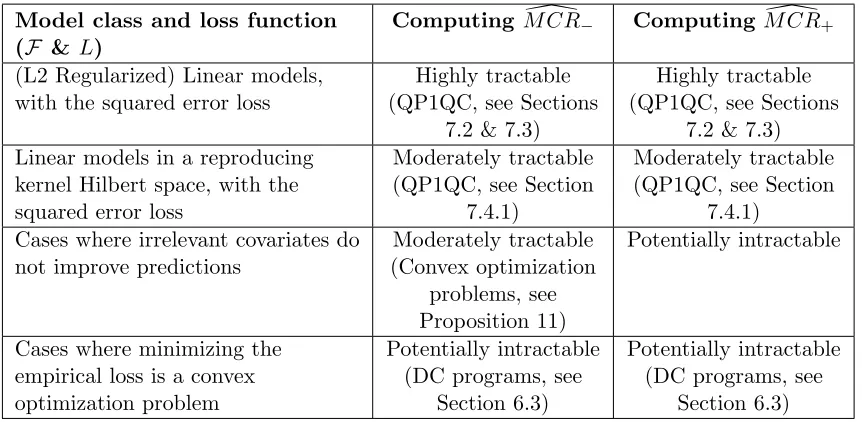
Model class and loss function (_F &L)

Computing M CR\− Computing M CR\+

(L2 Regularized) Linear models, with the squared error loss

Highly tractable (QP1QC, see Sections

7.2 & 7.3)

Highly tractable (QP1QC, see Sections

7.2 & 7.3) Linear models in a reproducing

kernel Hilbert space, with the squared error loss

Moderately tractable (QP1QC, see Section

7.4.1)

Moderately tractable (QP1QC, see Section

7.4.1) Cases where irrelevant covariates do

not improve predictions

Moderately tractable (Convex optimization

problems, see Proposition 11)

Potentially intractable

Cases where minimizing the empirical loss is a convex optimization problem

Potentially intractable (DC programs, see

Section 6.3)

Potentially intractable (DC programs, see

Section 6.3)

Table 1: Tractability of empirical MCR computation for different model classes – For each

case, we describe the tractability of computing M CR\− and M CR\+ using our

proposed approaches. Computing empirical MCR can be reduced to a sequence of optimization problems, the form of which are noted in parentheses within the above table.

computing M CR\−() only requires that we minimize convex combinations of ˆeorig(f) and

ˆ

eswitch(f), which is no more difficult than minimizing the average loss over an expanded and

reweighted sample (See Eq 6.2 & Proposition 11).

ComputingM CR\+() however will require that we are able to minimize arbitrary linear

combinations of ˆeorig(f) and ˆeswitch(f). In Section 6.3, we outline how this can be done for

convex model classes – classes for which the loss function is convex in the model parameter.

Later, in Section 7, we give more specific computational procedures for whenF is the class

of linear models, regularized linear models, or linear models in a reproducing kernel Hilbert space (RKHS). We summarize the tractability of computing empirical MCR for different model classes in Table 1.

To simplify notation associated with the reference modelfref, we present our

computa-tional results in terms of bounds on empirical MR subject to performance thresholds on the

absolutescale. More specifically, we present bound functionsb−andb+satisfyingb−(abs)≤ d

M R(f)_≤b+(abs) simultaneously for all{f, abs : ˆeorig(f)≤abs, f ∈ F, abs>0}(Figures

2 & 8 show examples of these bounds). The binary search procedures we propose can be

used to tighten these boundaries at a particular valueabs of interest.

We briefly note that as an alternative to the global optimization procedures we discuss below, heuristic optimization procedures such as simulated annealing can also prove useful

in bounding empirical MCR. By definition, the empirical MR for any model in ˆ_R() forms

a lower bound for M CR\+(), and an upper bound forM CR\−(). Heuristic maximization

Throughout this section, we assume that 0 < minf∈Feˆorig(f), to ensure that MR is

finite.

6.1. Binary Search for Empirical MR Lower Bound

Before describing our binary search procedure, we introduce additional notation used in

this section. Given a constant γ _∈ R and prediction model f _{∈ F}, we define the linear

combination ˆh−,γ, and its minimizers (for example, ˆg−,γ,F), as

ˆ

h−,γ(f) :=γeˆorig(f) + ˆeswitch(f), and gˆ−,γ,F ∈arg min

f∈F

ˆ

h−,γ(f).

We do not require that ˆh−,γ is uniquely minimized, and we frequently use the abbreviated

notation ˆg−,γ when F is clear from context.

Our goal in this section is to derive a lower bound on M Rd for subsets ofF in the form

of _{f _{∈ F} : ˆeorig(f) ≤ abs}. We achieve this by minimizing a series of linear objective

functions in the form of ˆh−,γ, using a similar method to that of Dinkelbach (1967). Often,

minimizing the linear combination ˆh−,γ(f) is more tractable than minimizing the MR ratio

directly.

Almost all of the results shown in this section, and those in Section 6.2, also hold if we

replace ˆeswitch with ˆedivide throughout (see Eq 3.5), including in the definition of M Rd and

ˆ

h−,γ(f). The exception is Proposition 11, below, which we may still expect to approximately

hold if we replace ˆeswitch with ˆedivide.

Given an observed sample, we define the following condition for a pair of values_{γ, abs} ∈

R×R>0, and argmin function ˆg−,γ:

Condition 8 (Criteria to continue search for M Rd lower bound) ˆh−,γ(ˆg−,γ) ≥ 0 and

ˆ

eorig(ˆg−,γ)≤abs.

We are now equipped to determine conditions under which we can tractably create a lower bound for empirical MR.

Lemma 9 (Lower bound for M Rd) Ifγ _∈Rsatisfies hˆ−,γ(ˆg−,γ)≥0, then

ˆ

h−,γ(ˆg−,γ)

abs −

γ ≤M Rd(f) (6.1)

for all f ∈ F satisfyingeˆorig(f)≤abs. It also follows that

−γ _≤M Rd(f) for allf _{∈ F}.

Additionally, if f = ˆg−,γ and at least one of the inequalities in Condition 8 holds with equality, then Eq 6.1 holds with equality.

Lemma 9 reduces the challenge of lower-bounding M Rd(f) to the task of minimizing

the linear combination ˆh−,γ(f). The result of Lemma 9 is not only a single boundary for

a particular value of abs, but a boundary function that holds all values of abs >0, with

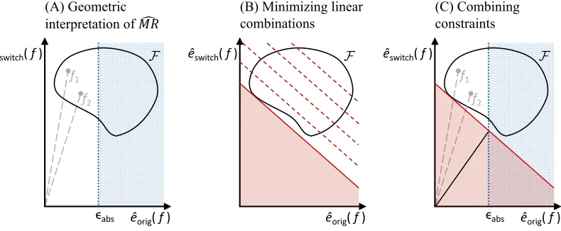
f1

f2 êswitch( f )

êorig( f ) ϵabs

(A) Geometric interpretation of !"#

F êswitch( f )

êorig( f ) (B) Minimizing linear combinations

F

f1

f2

êswitch( f )

êorig( f )

ϵabs

(C) Combining constraints

F

Figure 4: Above, we illustrate the geometric intuition for Lemma 9. In Panel (A), we show

an example of a hypothetical model classF, marked by the enclosed region. For

each model f _{∈ F}, the x-axis shows ˆeorig(f) and the y-axis shows ˆeswitch(f).

Here, we can see that the condition minf∈Fˆeorig(f)>0 holds. The blue dotted

region marks models with higher empirical loss. We mark two example models

within _F as f1 and f2. The slopes of the lines connecting the origin to f1 and

f2 are equal to M Rd(f1) and M Rd(f2) respectively. Our goal is to lower-bound

the slope corresponding to M Rd for any model f satisfying ˆeorig(f) ≤ abs. In

Panel (B), we consider the linear combination ˆh−,γ(f) = γeˆorig(f) + ˆeswitch(f)

for γ = 1. Above, contour lines of ˆh−,γ are shown in red. The solid red line

indicates the smallest possible value of ˆh−,γ across f ∈ F. Specifically, its

y-intercept equals minf∈Fˆh−,γ(f). If we can determine this minimum, we can

determine a linear border constraint on F, that is, we will know that no points

corresponding to modelsf _{∈ F} may lie in the shaded region above. Additionally,

if minf∈Fˆh−,γ(f)≥0 (see Lemma 9), then we know that the origin is either

excluded by this linear constraint, or is on the boundary. In Panel (C), we

combine the two constraints from Panels (A) & (B) to see that models f _{∈ F}

satisfying ˆeorig(f)≤abs must correspond to points in the white, unshaded region

above. Thus, as long as the unshaded region does not contain the origin, any

line connecting the origin to the a modelf satisfying ˆeorig(f)≤abs (for example,

here,f1,f2) must have a slope at least as high as that of the solid black line above.

It can be shown algebraically that the black line has slope equal to the left-hand

side of Eq 6.1. Thus the left-hand side of Eq 6.1 is a lower bound forM Rd(f) for

In addition to the formal proof for Lemma 9, we provide a heuristic illustration of the result in Figure 4, to aid intuition.

It remains to determine which value ofγ should be used in Eq 6.1. The following lemma

implies that this value can be determined by a binary search, given a particular value of

interest for abs.

Lemma 10 (Monotonicity forM Rd lower bound binary search) The following monotonicity results hold:

1. ˆh−,γ(ˆg−,γ) is monotonically increasing in γ.

2. eˆorig(ˆg−,γ) is monotonically decreasing in γ.

3. Givenabs, the lower bound from Eq 6.1,

n_ˆh

−,γ(ˆg−,γ)

abs −γ o

, is monotonically decreasing

in γ in the range where eˆorig(ˆg−,γ)≤abs, and increasing otherwise.

Given a particular performance level of interest, abs, Point 3 of Lemma 10 tells us that

the value of γ resulting in the tightest lower bound from Eq 6.1 occurs when γ is as low as

possible while still satisfying Condition 8. Points 1 and 2 show that ifγ0 satisfies Condition

8, and one of the equalities in Condition 8 holds with equality, then Condition 8 holds for

all γ _≥γ0. Together, these results imply that we can use a binary search to determine the

value of γ to be used in Lemma 9, reducing this value until Condition 8 is no longer met.

In addition to the formal proof for Lemma 10, we provide an illustration of the result in Figure 5 to aid intuition.

Next we present simple conditions under which the binary search for values of γ can be

restricted to the nonnegative real line. This result substantially extends the computational

tractability of our approach, as minimizing ˆh−,γ for γ ≥ 0 is equivalent to minimizing a

reweighted empirical loss over an expanded sample of sizen2_:

ˆ

h−,γ(f) =γˆeorig(f) + ˆeswitch(f) =

n X

i=1 n X

j=1

wγ(i, j)L{f,(y[i],X1[j,·],X2[i,·])}, (6.2)

wherewγ(i, j) = γ1(i=j)_n +_n(n1(i6=j)₋₁₎ ≥0.

Proposition 11 (Nonnegative weights for M Rd lower bound binary search) Assume that L

and _F satisfy the following conditions.

1. (Predictions are sufficient for computing the loss) The loss L_{f,(Y, X1, X2)} depends on the covariates(X1, X2)only via the prediction functionf, that is,L{f,(y, x(a)1 , x

(a) 2 )}=

L_{f,(y, x(b)₁ , x(b)₂ )_} whenever f(x(a)₁ , x(a)₂ ) =f(x(b)₁ , x(b)₂ ).

2. (Irrelevant information does not improve predictions) For any distribution D satisfy-ing X1 ⊥D (X2, Y), there exists a function fD satisfying

EDL{fD,(Y, X1, X2)}= min

f∈FEDL{f,(Y, X1, X2)},

and

fD(x (a)

1 , x2) =fD(x (b)

1 , x2) for anyx (a) 1 , x

(b)

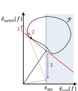
F êswitch( f )

êorig( f )

ϵabs

1 ₂

3

Figure 5: Monotonicity for binary search. Above we show a version of Figure 4-C for two

alternative values ofγ. This figure is meant to add intuition for the monotonicity

results in Lemma 10, in addition to the formal proof. Increasing γ is equivalent

todecreasing the slope of the red line in Figure 4-C. We define two values γ1 <

γ2, where γ1 corresponds to the solid red line, above, and γ2 corresponds to

the semi-transparent red line. The y-intercept values of these lines are equal to ˆ

h−,γ1(ˆg−,γ1) and ˆh−,γ2(ˆg−,γ2) respectively (see Figure 4-C caption). The solid and

semi-transparent black dots mark ˆg−,γ1 and ˆg−,γ2 respectively. Pluggingγ1andγ2

into Eq 6.1 yields two lower bounds forM Rd, marked by the slopes of the solid and

semi-transparent black lines respectively (see Figure 4-C caption). We see that

(1) ˆh−,γ1(ˆg−,γ1) ≤ ˆh−,γ2(ˆg−,γ2), that (2) ˆeorig(ˆg−,γ1) ≥ ˆeorig(ˆg−,γ2), and that (3)

the left-hand side of Eq 6.1 is decreasing inγ when ˆeorig(ˆg−,γ)≤abs. These three

conclusions are marked by arrows in the above figure, with numbering matching the enumerated list in Lemma 10.

Letγ = 0. Under the above assumptions, it follows that either (i) there exists a functionˆg−,0 minimizingˆh−,0 that does not satisfy Condition 8, or (ii)eˆorig(ˆg−,0)≤absandM Rd(g−,0)≤

1 for any function ˆg−,0 minimizing hˆ−,0.

The implication of Proposition 11 is that, when the conditions of Proposition 11 are met,

the search region forγ can be limited to the nonnegative real line, and minimizing ˆh−,γ will

be no harder than minimizing a reweighted empirical loss over an expanded sample (Eq 6.2).

To see this, recall that for a fixed value ofabs we can tighten the boundary in Lemma 9 by

conducting a binary search for the smallest value of γ that satisfies Condition 8. If setting

γ equal to 0 does not satisfy Condition 8, and the search for γ can be restricted to the

nonnegative real line, where minimizing ˆh−,0 is more tractable (see Eq 6.2). Alternatively,

if ˆeorig(g−,0) ≤ abs and M Rd(g−,0) ≤ 1, then we have identified a well-performing model

g−,0 with empirical MR no greater than 1. For abs = ˆeorig(fref) +, this implies that

\

M CR−()≤1, which is a sufficiently precise conclusion for most interpretational purposes