Smart Algorithms to Control a Variable Speed Wind Turbine

* Corresponding author.

E-mail addresses: [email protected] (Nabil

Farhane), [email protected] (Ismail Boumhidi),

[email protected] (Jaouad Boumhidi).

DOI: 10.9781/ijimai.2017.08.001

Keywords

Adaptive Fuzzy Neural Network Sliding Mode (AFNNSM), Sliding Mode Control (SMC), Particle Swarm Optimization (PSO), Variable Speed Wind Turbine.

Abstract

In this paper, a robust adaptive fuzzy neural network sliding mode (AFNNSM) control design is proposed to maximize the captured energy for a variable speed wind turbine and to minimize the efforts of the drive shaft. Fuzzy neural network (FNN) is used to improve the mathematical system model, by the prediction of model unknown function, which is used by the Sliding mode control approach (SMC) and enables a lower switching gain to be used despite the presence of large uncertainties. As a result, the used robust control action did not exhibit any chattering behavior. This FNN is trained on-line using the backpropagation algorithm (BP). The particle swarm optimization (PSO) algorithm is used in this study to optimize the learning rate of BP algorithm in order to improve the network performance in term of the speed of convergence. The stability is shown by the Lyapunov theory and the trajectory tracking errors converge to zero without any oscillatory behavior. Simulations illustrate the effectiveness of the designed method.

Smart Algorithms to Control a Variable Speed Wind

Turbine

Nabil Farhane

1

_{, Ismail Boumhidi}

1

_{, Jaouad Boumhidi}

2

_*

1

_{LESSI Laboratory, Department of Physics, Faculty of Sciences, Sidi Mohammed Ben Abdellah, Fez, (Morocco)}

2

_{LIIAN Laboratory, Department of Computer Science, Faculty of Sciences Sidi Mohammed Ben}

Abdellah, University of Fez (Morocco)

Received 2 June 2017 | Accepted 15 July 2017 | Published 21 August 2017

I.

Introduction

W

ind energy is an abundant renewable source of new electrical generation capacity in the world, and it is exploited by converting the kinetic energy of moving air mass into electricity; therefore, it is necessary to introduce tools to make these installations

more profitable [1]. Practically, there are two main types of horizontal

axis wind turbines: fixed speed and variable speed [2]. In this study, we consider the case of variable speed, due to its great ability in the extraction of energy. In addition to that, variable speed system is more

complex and requires an efficient control strategy [3]. Several studies have been devoted to the control of the aeroturbine mechanical as well as the electrical components. This work is devoted to the mechanical part (aeroturbine), with the main objective of designing a controller in order to maximize the energy captured from the wind and minimize the stress on the drive train shafts that takes into consideration the nonlinear

nature of the system behavior and the flexibility of the drive-train shaft.

The proposed control structure also overcomes the drawbacks of some existing control methods.

The sliding mode control [4-7], is widely used in the control of a variable speed wind turbine. This is due to its property of robustness with respect to uncertainties and disturbances [8],[9]. The chattering behavior is especially the main problem in the design of SMC.

One possible method to solve this problem is the boundary layer approach [6]. This technique has given good results when the system uncertainties are small. However, when these uncertainties are large, a high gain is needed and higher amplitude of chattering is produced. In order to solve this problem, we proceed to use FNN for the estimation of the unknown model function so that the system uncertainties can be kept small and hence enable a lower switching gain to be used. The designed method is a combination of traditional SMC and FNN with online adaptation of the parameters.

Intelligent systems such as fuzzy systems and neural networks are being used successfully in an increasing number of application areas [10]-[14]-[23]. Fuzzy neural networks (FNNs) have the low-level learning and computation power of neural networks, and the high-level human-like thinking and reasoning of fuzzy theory. The proposed control consists of the so called equivalent control added with robust control term, the FNN predicted unknown terms are incorporated in the equivalent control component, thus enable the robust component to be used with a small gain which is responsible to compensate the network errors prediction. The FNN is trained on-line using the backpropagation algorithm (BP). The learning rate is one of the parameters of BP algorithm which have a significant influence on results; learning rate which is too small or too large may not be favourable for convergence. Particle swarm optimization (PSO) algorithm is used in this work to optimize this parameter in order to improve the training speed.

II.

Wind Turbine Modelization

Wind energy across a surface

A

_v depends on the cube of the wind speed

v

, and the density of the air

ρ

. This energy is given by:

3

2

1

v

v

A

P

_v

=

ρ

(1)

where:

2

R

A

_v

=

π

₍₂₎

R

is the radius of the rotor. A variable speed wind turbine is composed of aeroturbine, a gearbox, and a generator. The aerodynamic power captured by the rotor is given as follows:

Pa= R Cp

( )

v 1

2

2 3

ρπ λ β,

(3)

Where

C

_p is the power coefficient,

β

is the pitch angle and the tip-speed ratio,

λ

, is given as follows:

v

R

r

ω

λ =

(4)

With

ω

r is the rotor speed. By using the relationship:

a r

a

T

P

=

ω

₍₅₎

The aerodynamic torque expression is:

(6)

Where:

( )

( )

λ

β

λ

β

λ

, p ,

q

C

C =

₍₇₎

( )

λ

,

β

q

C

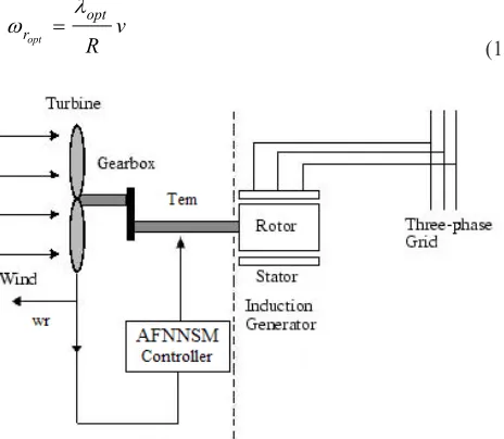
is the torque coefficient.

In the literature, the wind turbine is presented by the modelling of the mechanical part [15]-[17], or by that of the electrical part [18], [19]. In this paper, we are interested in the modelling of the mechanical part of the variable speed wind turbine, which is presented by a two-mass model that is shown in Fig. 1.

The dynamics of the rotor is characterized by a differential equation of the first order:

(8)

r

J

and

K

_r are respectively the rotor inertia and the rotor friction coefficient.

The low-speed shaft torque resulting effects of friction and torque generated by the differences between the rotor angular velocity

r

ω

and that of the output shaft (see Fig. 1):

(9)

and are respectively the shaft stiffness coefficient and the shaft damping coefficient.

r

θ

_and

are respectively the rotor side angular deviation and the gearbox side angular deviation.

The relationship between the high-speed shaft torque and the generator electromagnetic torque is given by:

(10)

g

J

,

ω

_g and

K

_g are respectively the generator inertia, the generator speed and the generator friction coefficient. Let’s assume an ideal gearbox with transmission ratio

n

_g, we get:

(11)

g

θ

is the generator side angular deviation.

Fig. 1. Two-mass model of wind turbine.

Replacing the time derivative of from (9) and using (10) and (11) we get the following dynamic system model (12) :

The nonlinear character of this system is due to the aerodynamic torque as follows:

(12)

This depends on a strongly nonlinear way, the rotor speed

ω

_r, the blade pitch angle

β

and the wind speed

v

which is a not controllable input, random and strongly fluctuating.

III.

Design of The Fuzzy Neural Network Sliding Mode

Control

The main control objective is to maximize the captured wind energy and minimize the efforts of drive train shafts. The power coefficient

curve

C

_p

( )

λ,

β

has a unique maximum which corresponds to the optimal wind energy [20]:

(

opt opt

)

p_opt

p

C

C

λ

,

β

=

(13)

The rotor, thus, provides maximum aerodynamic power, only to the

tip-speed

λ

_opt:

v

R

opt r opt

ω

λ

=

(14)

To maximize the captured energy of the wind, the variables

λ

and

β

must be maintained at their optimal values in order to ensure maximum value of

C

_p. So, the blade pitch angle is fixed at its optimal value

β

opt. The tip-speed

λ

depends on both of the wind speed

v

and the rotor speed

ω

_r. As the wind speed is not a controllable input, the rotor speed

ω

_r must be adjusted by (As seen in Fig. 2), to track the optimal reference given by:

v

R

opt ropt

λ

ω

=

(15)

Fig. 2. Basic configuration of wind turbine system.

A. Controller Design

Let define ,

x

₁

=

ω

_r and

x

₃

=

ω

_g, the dynamic system model described by (12) can be rewritten in the state space as follows:

(16)

R

u

∈

and y∈R are respectively the input and the output of the system, is the state vector of the system which is assumed to be available for measurement, and f

(

x₁,x₂,x₃ is the nominal representation of the system given as:

(17)

represents the unknown model part of the system (uncertainties and external disturbances) and is known constant.

In the following, the tracking error is defined as:

opt r r

e

=

ω −

ω

(18)

The relative degree of the system (16) is

r

=

2

. The sliding variable can be defined as:

(

x

topt

) (

x

topt

)

e

e

S

=



+

γ

=

₂

−

ω



+

γ

₁

−

ω

₍₁₉₎

Where

γ

is a positive constant.

Differentiating

S

_{with respect to time, we have:}

(20)

where the function:

( ) (

x

t

f

x

x

x

)

x

(

)

d

( )

t

F

,

=

₁

,

₂

,

₃

+

γ

₂

−

ω



_topt

+

γ

ω



_topt

+

₍₂₁₎

The following condition (22) must be satisfied [6] to guarantee the existence of sliding mode in finite time:

S

S

S



<

−

η

(22)

Where

η

is a small positive constant. The control law that satisfies Eq. (20) is given by:

(23)

Where , with

F

ˆ

x

,

t

)

is the Fuzzy neural

S

sat

b

U

_s

=

−

α

(24)

Where

sat

(.)

is the saturation function given by:

(25)

L is the boundary layer thickness and

α

_{is chosen according to the}

following theorem.

The fuzzy neural network prediction error is denoted:

F

F

F

−

ˆ

=

ε

₍₂₆₎

With ε_F <ε*F and

ε

F* is the upper bound of the network error prediction assumed known.

The block diagram of the AFNNSM system is depicted in Fig. 3.

Fig. 3. Block diagram of the proposed AFNNSM control wind turbine.

Theorem: Consider the system described by (16) in the presence of large uncertainties. If the system control is designed as:

(27)

Where , with Fˆ

( )

x,t is the output of the proposed fuzzy neural network, ε*_F +η<α ; the trajectory tracking errors will converge to zero in finite time.

Proof: Consider the candidate Lyapunov function:

By replacing the expression of

u

_{given in the theorem we have:}

( ) ( )

(

F x,t Fˆ x,t sat(S)

)

S

V = − −

α

) ( ) ( ) (

* _{Ssat S}

S S Ssat F S S Ssat F S F

α

ε

α

ε

α

ε

− < − ≤ − =

By choosing

ε

*_F

+

η

<

α

we have: For any

L

>

0

, if S >L,

) ( )

(S sign S

sat = _{the function . However,}

in a small L-vicinity of the origin [6],

L S S

sat( )= is continuous, the system trajectories are confined to a boundary layer of sliding mode manifold S =0..

B. Fuzzy Neural Network Representation

In this paper, we consider a FNN with five-layered of adjustable weights (Fig. 4). The

{ }

x

_{i i=1,2} are input variables, Fˆ =ξˆ(x,t) is the output variable. Fig. 4 shows the structure of the FNN, which is comprised of the input, the membership, the rule, the normalized and the output layers. To give a clear understanding of the signal propagation and mathematical function in each layer, the following section describes FNN functions layer by layer.

Fig. 4. The architecture of the proposed fuzzy neural network for the prediction of uncertain part.

Layer 1: This layer, which corresponds to one input variable

)

2

,1

(

k

=

x

_k , only transmits input values to the next layer directly. Layer 2: In this layer, each node performs a membership function and acts as a unit of memory. The Gaussian function is adopted as the membership function. For the

kth

input, the corresponding net input and output of the

_lth

node can be expressed as:

]

)

(

)

(

exp[

)

(

₂ 2 l k l k k k l k

c

x

x

σ

µ

=

−

−

(28)

where

c

l_k and

σ

_kl ; l =1,2,,M are the mean and standard deviation of the Gaussian function of the

lth

partition for the

kth

input variable

x

k , respectively, and M is the total number of fuzzy

rules.

Layer 3: This layer represents one fuzzy logic rule and performs precondition matching of a rule.The output of a rule node in this layer is calculated by the product operation as follows.

)

(

)

(

2 1 k k l k l

x

=

∏

₌

µ

x

φ

(29)

Layer 4: In this layer, each of these firing strengths of the rules is compared with the sum of all the firing strengths. Therefore, the normalized firing strengths are computed in this layer as,

∑ = = M l l l l x x x

1 ( )

∑

=

=

M

l

w

l l

x

x

1

(

)

)

(

ˆ

_φ

ξ

The aim of the learning algorithm is to adjust the weights of

w

_ςlˆ,

l

c

_ς and

σ

ςl.The on-line learning algorithm is a gradient descent (GD)

search algorithm in the space of network parameters [21]. The essence of (GD) consists of iteratively adjusting the weights the direction opposite to the gradient of error, so as to reduce the discrepancy according to:

l F w

l l

w



=

η

ε

φ

₍₃₁₎

Where l y w

η

_{is the leaning rate for} l y

w

The updated laws of

c

ςl and

σ

ςl also can be obtained by the gradient

decent search algorithm:

2

)

(

)

(

2

_l k l k k l l F c l k

c

x

w

c

l

k

ε

φ

σ

η

−

=



3 2

)

(

)

(

2

_l k l k k l l F l k l

k

η

ε

φ

w

x

_σ

c

σ

σ

−

=



Where l k c

η

_and l k σ

η

_{are the learning-rate parameters of the mean}

and the standard deviation of the Gaussian functions.

C. Particle Swarm Optimization Algorithm

The objective is to optimize the learning rate

η

w_l by the PSO

algorithm.

In PSO, m particles fly through an n-dimensional search space. For each particle i, there are two vectors: the velocity vector

and the position vector

X

_i

=

(

x

_i1

,

x

_i2

,...,

x

_i

_n

)

. Similar to bird socking and fishes schooling, the particles are updated according to their previous best position and the whole swarm’s previous best position . This means that particle i adjusts its velocity

V

_i and position

X

_i in each generation according to the equations bellow [22]:

(32)

(33)

Where d =1,2,...,n;

c

₁

,

c

₂ are the acceleration coefficients with positive values, which we take as:

c

₁

=

1

and

c

₂

=

2

in this paper; rand

)

₁, rand

( )

₂ are random numbers between 0 and 1. The new velocity and position for each particle are calculated using the equations (32) and (33) based on its velocity , best position and the swarm’s best position .

In order to calculate the optimized parameter of learning rate

η

w_l

given in equation (29), the PSO is used on-line to minimize the neural network prediction error.

We define the quadratic errors as:

The objective function

f

to be minimized is chosen as the norm of the quadratic error: with the vector that contains all errors .

The PSO algorithm tests the search space using m particles

according to (30) and (31). Each particle i moves in search space and stores its best position , then, it compares all positions to finally take out the chosen

η

_k−_optimum that gives the minimum value of the

objective function

f

.

IV.

Simulation Results

Different simulation cases are considered for the case of a two-mass model of the wind turbine with:

• Presence of constant additive control disturbance

d

of 10 , • Presence of an additive measurement noise on

ω

g, with a SNR of

approximatively 7 .

• A wind speed profile of 7 m/s means value.

The two-mass model parameters are presented below:

Three membership functions have been used for each of the two inputs of the FNN. The associated fuzzy sets with Gaussian membership function for each input signal, have initial input for the mean and the standard deviation:

21.9693]

1.2640

[-6.4470

c

₁

=

2.1675]

0.0241

[0.0043

*

005

1.0e

1

=

+

σ

30.8045]

275.7842

-[-130.1245

c

₂

=

4.1794]

0.0261

[0.0140

*

005

1.0e

2

=

+

σ

The initial output weights :

118.3859] 119.7829 10.9070 - [ − =

w , being the initial

weights, which are obtained hors-line identification system.

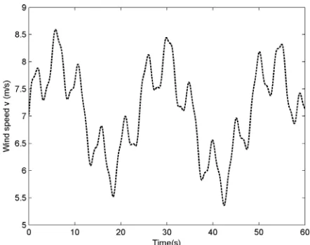
Fig. 5 presents the wind speed profile used in this study. Fig. 6 shows the estimation error for the predicting function F.

Fig. 5 is proposed for an average speed, it was considered the case where the wind speed is highly variable and the case where the wind speed does not change rapidly.

Fig. 6. Error estimation of the predicting function F.

Fig. 7. Rotor speed with α = 1.2.

To gain a large enough alpha = 1.2 we see the output controlled by the standard sliding mode converges slowly. However that commissioned by the proposed method NNSMC converges rapidly to the desired output

Fig. 8. Electromagnetic torque with α = 1.2.

Fig. 8 shows the actual and optimal trajectory of the rotor speed, we find that the best tracking performance is obtained when applying the RFNNSM.

Fig. 9. Rotor speed with α = 0.9.

For comparison we have considered in the control law, for both AFNNSM and traditional SMC controllers, the same gain α = 1.2(see the obtained outputs in Fig. 7) and α = 0.9 (see the obtained outputs in Fig. 9). From these figures, it can be seen that, the best tracking performance is obtained when the proposed AFNNSM controller is applied. The corresponding control signals are given in Fig. 8 for

α = 1.2, and in Fig. 10 for α = 0.8. Fig. 9 shows that the standard SMC controller totally failed to control the system.

Fig. 10. Electromagnetic torque with α = 0.9.

By using the a gain aloha = 0.9, Fig. 10 shows the optimal trajectory of the rotor speed, otherwise we find that the best tracking performance is obtained when the RFNNSM is applying.

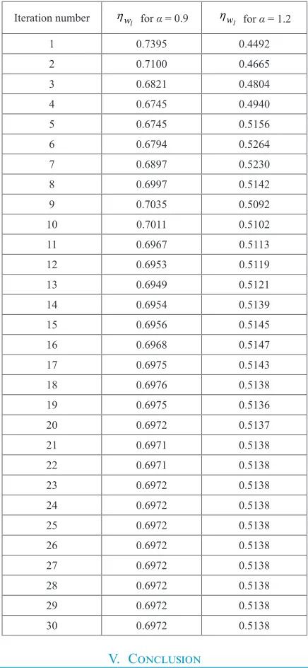
TABLE I. The Global Optimum Particle of Learning Rate

Iteration number ηw_l for α = 0.9 ηwl for α = 1.2

1 0.7395 0.4492

2 0.7100 0.4665

3 0.6821 0.4804

4 0.6745 0.4940

5 0.6745 0.5156

6 0.6794 0.5264

7 0.6897 0.5230

8 0.6997 0.5142

9 0.7035 0.5092

10 0.7011 0.5102

11 0.6967 0.5113

12 0.6953 0.5119

13 0.6949 0.5121

14 0.6954 0.5139

15 0.6956 0.5145

16 0.6968 0.5147

17 0.6975 0.5143

18 0.6976 0.5138

19 0.6975 0.5136

20 0.6972 0.5137

21 0.6971 0.5138

22 0.6971 0.5138

23 0.6972 0.5138

24 0.6972 0.5138

25 0.6972 0.5138

26 0.6972 0.5138

27 0.6972 0.5138

28 0.6972 0.5138

29 0.6972 0.5138

30 0.6972 0.5138

V.

Conclusion

This paper addressed the robust optimal reference tracking problem for a variable speed wind turbine. The designed method is a combination of traditional sliding mode control approach and fuzzy neural network. The later is employed to approximate the unknown nonlinear model function with online adaptation of parameters via BP learning algorithm. This provides a better description of the plant, and hence enables a lower switching gain to be used despite the presence of large uncertainties. The particle swarm optimization (PSO) algorithm is used to optimize the learning rate of BP algorithm in order to get faster convergence. The comparison with the traditional sliding mode control has been realized and simulation results have shown a good performance of the proposed method to track the optimal reference without any chattering problem.

References

[1] J. F. Manwell, J. G. McGowan, A. L. Rogers, Wind Energy Explained: Theory, Design and Applications (John Wiley & Sons, 2002).

[2] G. Ofualagba, E. U. Ubeku, Wind energy conversion system- wind turbine modelling, Power and Energy Society General Meeting - Conversion and Delivery of Electrical Energy in the 21st Century, IEEE, 2008, 1-8.

[3] T. Burton, D. Sharpe, N. Jenkins, E. Bossanyi, Wind Energy Handbook (John Wiley & Sons, 2001).

[4] S. Abdeddaim, A. Betka. Optimal Tracking and Robust Power Control of the Doubly Fed Induction Generator wind Turbine, Electric Power Systems Research, vol. 49, 2013, pp. 234–242.

[5] V. I. Utkin, Sliding Modes in Control Optimization (Springer-Verlag, 1992).

[6] J.J. Slotine, Sliding Controller Design for Non-linear Systems, International Journal of Control, vol. 40, n. 2, 1984, pp. 421–434.

[7] V. Utkin, J. Guldner, J. Shi, Sliding Mode Control in Electromechanical System (Taylor & Francis, London, 1999).

[8] P.F. Puleston, F. Valenciaga, Chattering Reduction in a Geometric Sliding Mode method. A Robust Low-chattering Controller for an Autonomous Wind System, Control and Intelligent Systems, vol. 37, n. 1, 2009, pp. 39-45.

[9] H. Amimeur , D. Aouzellag , R. Abdessemed, K. Ghedamsi, Sliding Mode Control of a Dual-stator Induction Generator for Wind Energy Conversion Systems, International Journal of Electrical Power and Energy Systems, vol. 42, n. 1, 2012, pp. 60–70.

[10] Y. C. Chen, C. C. Teng, A Model Reference Control Structure Using a Fuzzy Neural Network. Fuzzy Sets and Systems, vol. 73, n. 3, 1995, pp. 291–312.

[11] V. Gorrini, H. Bersini, Recurrent fuzzy systems. In Proceedings of the IEEE international conference on fuzzy systems, vol. 1, 1994, 193–198.

[12] F.B. Duh, C.T. Lin, Tracking a Maneuvering Target Using Neural Fuzzy Network, IEEE Transactions on Systems, Man, and Cybernetics, vol. 34, n. 1, 2004, pp. 16–33.

[13] C.F. Juang, C.H. Hsu, Temperature Control by Chip-implemented Adaptive Recurrent Fuzzy Controller Designed by Evolutionary Algorithm, IEEE Transactions on Circuits System, vol. 52, n. 11, 2005, pp. 2376–2384.

[14] S.J. Lee, C.L. Hou, A Neural-fuzzy System for Congestion Control in ATM Networks, IEEE Transactions on Systems, Man, and Cybernetics, vol. 30, n. 1, 2000, pp. 2–9.

[15] J.M. Rubio, & LT. Aguilar, Maximizing the Performance of Variable Speed Wind Turbine with Nonlinear Output Feedback Control, Procedia Engineering, vol. 35, 2012, pp. 31-40.

[16] L. Munteanu, A. L. Bratcu, N-A. Cutululis, E. Ceanga, Optimal Control of Wind Energy Systems, Advances in Industrial Control (Springer, 2008).

[17] J.F. Adrià, G.B. Oriol, S. Andreas, S. Marc, M. Montserrat, Modeling and Control of The Doubly Fed Induction Generator Wind Turbine, Simulation Modelling Practice and Theory, vol. 18, n. 9, 2010, pp. 1365–1381.

[18] Ph. Delarue, A. Bouscayrol, A. Tounzi, X. Guillaud, Modelling, Control and Simulation of an Overall Wind Energy Conversion System, Renewable Energy, vol. 28, n. 8, 2003, pp. 1169-1185.

[19] A. Gaillard, P. Poure , S. Saadate , M. Machmoum, Variable Speed DFIG Wind Energy System for Power Generation and Harmonic Current Mitigation, Renewable Energy, vol. 34, n.6, 2009, pp. 1545–1553.

[20] K. A. Stol, Geometry and Structural Properties for the Controls Advanced Research Turbine (CART) from Model Tuning (Subcontractor Report SR-500-32087, National Renewable Energy Laboratory, Golden, CO, September. 2004).

[21] D. E. Rumelhart, G. E. Hinton, R. J. Williams, Learning internal representations by error propagation. In D. E. Rumelhart, J. L. McClelland (Ed), Parallel Distributed Processing, (Cambridge, MA, (1): MIT Press, 1986, 318–362).

[22] M. A. Cavuslua, C. Karakuzub, Neural Identification of Dynamic Systems on FPGA with Improved PSO Learning. Applied Soft Computing, vol. 12, 2012, pp. 2707–2718.

Nabil Farhane

Nabil Farhane received his M.Sc. degree from Sidi Mohammed ben Abdellah University of Fez in 2011. He is currently pursuing the Ph.D. degree at Sidi Mohammed ben Abdellah University. His research interests include fuzzy logic, neural networks, non-linear control, etc.

Ismail Boumhidi

Ismail Boumhidi is a professor of electronics at the Faculty of Sciences, Fez, Morocco. He received his Ph.D. degree from Sidi Mohammed ben Abdellah University, Faculty of Sciences, in 1999. His research areas include adaptive robust control, multivariable non-linear systems and fuzzy logic control with applications.

Jaouad Boumhidi