The Thirty-Third AAAI Conference on Artificial Intelligence (AAAI-19)
Deictic Image Mapping: An Abstraction
for Learning Pose Invariant Manipulation Policies
Robert Platt, Colin Kohler, Marcus Gualtieri
College of Computer and Information Science, Northeastern University 360 Huntington Ave, Boston, MA 02115, USA
{rplatt,ckohler,mgualti}@ccs.neu.edu
Abstract
In applications of deep reinforcement learning to robotics, it is often the case that we want to learn pose invariant policies: policies that are invariant to changes in the position and ori-entation of objects in the world. For example, consider a peg-in-hole insertion task. If the agent learns to insert a peg into one hole, we would like that policy to generalize to holes pre-sented in different poses. Unfortunately, this is a challenge us-ing conventional methods. This paper proposes a novel state and action abstraction that is invariant to pose shifts called deictic image mapsthat can be used with deep reinforcement learning. We provide broad conditions under which optimal abstract policies are optimal for the underlying system. Fi-nally, we show that the method can help solve challenging robotic manipulation problems.
Introduction
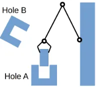
Policies learned by deep reinforcement learning agents are generally not invariant to changes in the position and ori-entation of the camera or objects in the environment. For example, consider the peg-in-hole insertion task shown in Figure 1. A policy that can insert the peg intoHole Adoes not necessarily generalize toHole B. In order to learn a pol-icy that can perform both insertions, the agent must be pre-sented with examples of the hole in both configurations dur-ing traindur-ing. This is a significant problem in robotics because we often want to learn policies most easily expressed relative to an object (i.e. relative to the hole) rather than relative to an image. Without the ability to generalize over pose, deep re-inforcement learning must be trained with experiences that span the space of all possible pose variation. For example, in order to learn an insertion policy for any hole configura-tion, the agent must be trained with task instances for hole configurations spanningSE(2), a three dimensional space. The problem is even worse inSE(3)which spans six dimen-sions. The need for all this training data slows down learning and hampers the agent’s ability to generalize over other di-mensions of variation such as task and shape. While pose invariance is not always desirable, the inability to generalize over pose can be a major problem.
This paper introduces deictic image mapping, an ap-proach to encoding robotic manipulation actions that
gen-Copyright c2019, Association for the Advancement of Artificial Intelligence (www.aaai.org). All rights reserved.
Figure 1: A policy for inserting a peg into Hole A learned using deictic image mapping generalizes to Hole B without any additional training.
eralizes over the pose of the robot and other objects in the world. We focus on the end-to-end learning setting in robotics where state is typically encoded in terms of im-ages and the action set corresponds to possible motions of the robot. Our key idea is to encode action as an image of the world that is centered, aligned, and focused on the target pose of the motion. Since this representation encodes motion actions in terms of the configuration of the world relative to the endpoint of the motion, it generalizes well over changes in object pose and camera viewpoint. We call this a “deictic” representation because motion actions are encoded relative to the environment rather than an absolute reference frame.
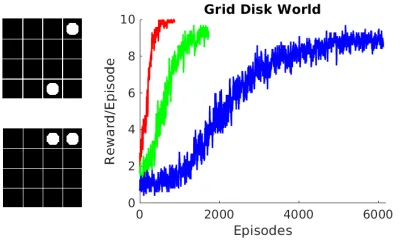
Figure 2: Left: the GRID-DISK domain. Disks are initially placed on a grid randomly (top left). The agent must pick one disk and place it adjacent to another (bottom left). Right: learning curves averaged over 10 runs for DQN applied to
GRID-DISKfor a3×3grid (red), a4×4grid (green), and a
5×5grid (blue).
Problem Statement
We will consider problems expressed for a class of robotic systems that we callmove-effectsystems.
Definition 1 (Move-Effect System). A move-effect system is a discrete time system comprised of a set of effectors mounted on a fully actuated platform that operates in a Eu-clidean space of dimensiond∈ {2,3}. On every time step, the system perceives an image or signed distance function,
I, and then executes a collision-free motion,am ∈ AM ⊂ SE(d), of the platform followed by a motion,ae ∈ AE, of
the effectors.
A good example of a move-effect robot is a robotic arm engaged in prehensile manipulation. The robot may move its hand (i.e. the “platform”) to any desired reachable pose
am∈ AM ⊂SE(3)via a collision-free motion. Once there,
it may execute an effector motionae∈ AEsuch as opening
or closing the hand. More complex manipulation systems can also be formalized this way. For example, a domestic robot that navigates within a house performing simple tasks can be expressed as a move effect system inSE(2)where the simple tasks to be performed are the “effector motions”.
Formulation as a Markov decision process
A Markov decision process (an MDP) is a tuple M = (S,A, T, R)whereS denotes a set of system states andA a discrete set of actions.T : S × A × S →[0,1]denotes the transition probability function where T(st, at, st+1)is
the probability of transitioning to statest+1when actionat
is taken from statest.R:S × A →Rdenotes the expected reward of executing actiona from states. The solution to an MDP is a control policyπ :S → Athat maximizes the expected sum of future discounted rewards when acting un-der the policy. We will assume that a motion planner (e.g. an RRT or trajectory optimization planner) is available that can find a collision free path to any reachable pose.
In order to use the MDP framework for move-effect sys-tems, we need to define state and action sets. An action is de-fined to be a pair,a= (am, ae)∈ AwhereA=AM× AE.
The agent does not observe state directly, but it can observe an imageI∈[0. . .216]|grid|=I, taken at the beginning of each time step taken via a camera and/or depth sensor. Here,
grid ⊂ Rd denotes the positions of a finite set of points corresponding to the pixels or voxels in the image or signed distance function. The system also has access to the config-uration of its effectors,θ∈Θ, obtained using joint position sensors. We define state to be a history of thekmost recent observations and actions:
st=hIt1−k, θ
1−k t , a
1−k
t , . . . , I−
1
t , θ−
1
t , a−
1
t , It, θti, (1)
whereItandθtdenote the current values for those two
vari-ables andIt−i,θ− i
t , anda− i
t denote the respective variables
as they wereitime steps in the past (i.e.itime steps prior tot).S =Ik×Θk× Ak−1is the set of all states. History
based representations of state as in Equation 1 are often used in deep reinforcement learning (e.g. (Mnih et al. 2013)).
Why move-effect problems are challenging
The standard MDP formulation described in the previous section is not well suited to move-effect systems. For exam-ple, consider theGRID-DISKdomain as shown in Figure 2, where the argent must pick one disk and place it horizon-tally adjacent to the other. Transitions are deterministic: a pick (resp. place) succeeds if executed for an occupied (resp. unoccupied) cell and does not otherwise. This example is a move-effect system where AM ⊂ SE(2) is the set of 16
grid positions and AE contains exactly one pick and one
place action (32 actions total). On each time step, the agent observes an image of the grid as well as a single bit that de-notes the configuration of its hand – either open or closed (Equation 1 fork = 1). Using DQN on the MDP formu-lation described above, the number of episodes needed to learn a good policy increases as the number of cells in the grid increases, as shown in Figure 2, right. In this experi-ment, we used a standard-greedy DQN with dueling net-works (Wang et al. 2015), no prioritized replay (Schaul et al. 2015), a buffer size of 10k, a batch size of 10, and an episode length of 10 steps. Epsilon decreased linearly from 100% to 10% over the training session. The neural network has two convolutional+relu+pooling layers of 16 and 32 units respectively with a stride of 3 followed by one fully con-nected layer with 48 units. We use the Adam optimizer with a learning rate of 0.0003.
Deictic image mapping
Move-effect systems have structure that makes problems in-volving these systems easier to solve than the results in Fig-ure 2 suggest. Notice that in the case ofGRID-DISK, the
2015). DDPG could make it easier for the agent to learn to generalize over position, but it cannot generalize over orien-tation. Instead, we introduce deictic image state and action mappings that induce an abstract MDP that captures prob-lem symmetries and can be solved using DQN.
Action mapping
As expressed in the Problem Statement, each action is a pair,
at =ham(t), ae(t)i ∈ A=AM × AE, where we use the
notation am(t) to describe the destination of the platform
motion andae(t)to describe the effector motion at timet.
Our key idea is to expressamin terms of the appearance of
the world in the vicinity ofamrather than as coordinates in
a geometeric space. Recall that on each time step, the move-effect system observes an image or signed distance function,
I ∈ I = [0. . .216]|grid|, expressed over a finite set of po-sitions,grid ⊂ Rd, corresponding to pixels or voxels. Let crop(I, am)⊂ Idenote a cropped region ofIcentered on amand aligned with the basis axes ofamand letI0denote
the space of all possible crops. The action mapping is then
gs:A → A0=I0× AEwhere:
gst(at) =hcrop(It, am(t)), ae(t)i, (2)
It is an element of st, and am(t) andae(t) are elements
ofat. We call this adeictic imageaction mapping because
it uses an image to encode the motion relative to other ob-jects in the world. This can be viewed as an action abstrac-tion (Ravindran 2004; Ravindran and Barto 2003) and we will callA0theabstract actionset. This encoding works well
for move-effect problems where the outcome of an effect ac-tion depends only on the local geometry of the world where the action was executed.
State mapping
The action mapping of Equation 2 induces a state abstrac-tion. Recall that we defined state to be the history of the last
k observations and actions (Equation 1). We can simplify this representation by using the action abstraction of Equa-tion 2. The easiest way to do this is to define abstract state to be the current robot state paired with a history of thek−1
most recently executed abstract actions:
fk(st) =h{ crop(It1−k, a1m−k(t)), a1e−k(t), . . . ,
crop(It−1, a−m1(t)), a−e1(t), θti (3)
whereIt−i,a−i
m(t), anda−ei(t)are elements ofstandS0 =
I0k−1× Ak−1
E ×Θis the set of abstract states. Whenkis
understood, we will sometimes abbreviatef =fk. We refer
toS0as theabstract state set.
DQN in the abstract state and action space
The state and action mappings introduced above induce an abstract MDP that can be solved using DQN. Let Q0 :
S0× A0 →
Rdenote the abstract action-value function, ex-pressed over the abstract state and action space, encoded by a deep neural network. At the beginning of each time step, we evaluate the abstract state,s0t = f(st), for the current
state,st. We can calculate the greedy action for the current
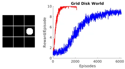
Figure 3: Left: example of a deictic action representation. Right: deictic (red) versus DQN baseline (blue) for5×5 GRID-DISK.
statestwith respect to the abstract action-value functionQ0
using:
a∗= arg max a∈AQ
0(f(s
t), gst(a)). (4)
After each time step, we store the underlying transition,
(st, at, st+1, rt)in the standard way. Training is nearly the
same as usual except that after sampling a mini-batch, we calculate targets using the abstract state-action value func-tion, rt + maxa∈AQ0(f(st), gst(a)), rather than in the standard way. The neural network that encodes Q0 takes an abstract state-action pair as input and outputs a sin-gle estimate of value. In our experiments, we use a stan-dard convolutional architecture comprised of two convolu-tion+relu+pooling layers followed by fully connected lay-ers.
Consider the following example of deictic image map-ping for the GRID-DISK domain introduced earlier. Recall that for an imageI ∈ I and a platform motionam ∈ AM, crop(I, am)is a cropped region ofI centered and aligned
witham.AM is the set of platform motion target locations
corresponding to the cells (|AM|= 16for4×4GRID-DISK).
In this example, we definecrop(I, am)to be the3×3cell
square region centered onam. (We use zero-padding foram
positions on near the edge of the grid.) For example, Fig-ure 3 left showscrop(I, am)for the place action shown in
Figure 2b. Since the agent is to place a disk to the left of an existing disk, the deictic image for this place action shows the existing disk to the right of an empty square where the place will occur. θ is the configuration of the effector: in this case just the configuration of the gripper jaws. Figure 3 right compares learning curves for DQN with deictic image states and actions versus the DQN baseline averaged over 10 runs each for the5×5GRID-DISKdomain. DQN is param-eterized just as it was in the last section. Notice that deictic image mapping speeds up learning considerably.
Scaling up
potential actions. One approach to handling this would be to adapt an actor critic method such as DDPG to the deictic im-age mapping setting. However, we have so far only explored the DQN version of our approach and leave an actor critic version for future work. Instead, this section introduces sev-eral techniques that together enable us to handle the large branching factor for problems in SE(2). Note that large ac-tion spaces are becoming more common in the literature. For example, (Li, Hsu, and Lee 2018) uses a hand-coded heuris-tic to prune action choices and (Zeng et al. 2018) uses a fully convolutional network architectures to evaluate Q-values for millions of actions.
Passing multiple actions as a batch to the Q-network: Perhaps the easiest way to handle the large number of ac-tions is to pass a large set of action candidates to the Q-network as a single batch. Neural Q-network back-ends such as TensorFlow are designed for this and it enables us to eval-uate as many as 4.6k actions in a single forward pass on a standard NVIDIA 1080 GPU.
Keeping an estimate of the state-value function:The large action branching factor is a problem every time it is nec-essary to evaluatemaxa∈AQ0(f(st), gst(a)). This happens twice in DQN: once during action selection and again dur-ing traindur-ing when evaluatdur-ing target values for a mini-batch. We eliminate the second evaluation by estimating the ab-stract state-value function,V0, concurrently with the abstract action-value function,Q0, using a separate neural network.
V0is trained using targets obtained during action selection: each time we select an action for a given state, we update theV0 network using the just-evaluated max for that state.
This enables us to calculate a target usingrt+γV0(f(st+1))
rather thanrt+γmaxa∈AQ0(f(st), gst(a)).
Value function hierarchy:Another way to speed up eval-uation of maxa∈AQ0(f(st), gst(a)) is to leverage a hier-archy of value functions specifically designed for move-effect problems inSE(2)(Gualtieri and Platt 2018). Rather than estimating Q0 directly using a single neural network, we use a hierarchy of two networks,Q01 andQ02(although one could envision additional levels of hierarchy). Q0
2 is
trained in the standard way: for each s, a pair in a mini-batch,Q02(f(s), gs(a))is trained with the corresponding
tar-get. However, we also trainQ01(f(s), gs(F ix(a)))with the
same target, whereF ix(a)∈SE(2)denotes the pose with the same position asabut with an orientation that is fixed with respect to the platform reference frame. Essentially, the
Q01estimate is an average of the value function over all
ori-entations for each given position.
Instead of maximizing by evaluating Q0
2 for the
posi-tion and orientaposi-tion of all possible moposi-tion acposi-tions, we score each position usingQ01and then maximizeQ02over the po-sitions and orientations corresponding to the top scoring positions under Q01. This is essentially a graduated non-convexity method (Blake and Zisserman 1987). First, we evaluate Q01(f(s), gs(¯a)) over all positions, ¯a ∈ A¯ =
{F ix(a) : a ∈ A}. Let A¯top denote the top scoring η percent of the abstract actions in A. Then, we evalu-¯ atemaxa∈A¯topQ02(f(s), gs(F ix−1(a))), whereF ix−1
de-notes the one-to-many inverse ofF ixthat returns all fully-specified poses that correspond to positions inA¯top. This
ap-proach enables us to estimate the maximum ofQ02without
exhaustively evaluating the function for all poses inSE(2). Like all graduated non-convexity methods, this approach is not guaranteed to provide an optimum. However, our results indicate that it works reasonably well on our problems (see the comparison in the next section).
Using hand-coded heuristics: Another way to reduce the action branching factor is to encode human knowledge about which kinds of motions are likely to be relevant to the prob-lem. This type of approach has been used by others includ-ing (Li, Hsu, and Lee 2018) who hand-coded a heuristic for identifying which push actions. In this paper, we con-strain the system to move only to positions that are within a neighborhood of some other visible object: we discard all motions, am, where the associated cropped image patch, crop(I, am), does not include pixels with some positive
height above the table plane.
Curriculum learning: Another thing that can speed up training is curriculum learning (Bengio et al. 2009). This ba-sically amounts to training the agent to solve a sequence of progressively more challenging tasks. The hard part is defin-ing the task sequence in such a way that each task builds upon knowledge learned in the last. However, this is par-ticularly easy with deictic image mapping. In this case, we just need to vary the discretization ofAM on each
curricu-lum task, starting with a coarse and ending with a fine dis-cretization. For example, suppose we want to learn aGRID
-DISKpolicy over a fine grid of possible disk locations. We would initially train using a coarse discretization and subse-quently train on a more fine discretization. Although some of the image patches in the fine discretization will be differ-ent from what was experienced in the coarse discretization, these new image patches will have a similar appearance to nearby patches in the coarse discretization. Essentially, plat-form motions that move to similar locations will be repre-sentated by similar image patches. As a result, policy knowl-edge learned at a coarse level will generalize appropriately at the fine level.
Experiments
We evaluate deictic image mapping in simulation and on a robot for problems with an action set that spansSE(2).
Block alignment in simulation
Curriculum stage number 1 2 3 4 5 6 7 8 Object Type Disks Disks Blocks Blocks Blocks Blocks Blocks Blocks
Num Positions 25 25 25 25 81 289 841 841
Num Orientations 2 8 2 4 8 8 8 16
Num Actions 100 400 100 200 1.2k 4.6k 13.5k 26.9k
Table 1: Eight-stage curriculum used in the simulated experiments.
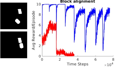
Figure 4: Left: block alignment problem. Top left: two blocks are placed randomly. Bottom left: the agent must pick up one block and place it roughly in alignment with the sec-ond. Right: learning curves for simulated blocks world do-main. Blue: DIM with hierarchical value function only in last two curriculum steps. Red: DQN baseline.
(1) Comparison with a DQN baseline: Here, we follow the eight-task curriculum shown in Table 1, starting with a task involving disks as in Figure 2 and ending with the block alignment task. During the first six stages of curricu-lum learning, we use all of the scaling-up techniques de-scribed in the last section except for the value function hi-erarchy (as we show later, this slows learning performance). We only turn on the value function hierarchy in the last two stages because the NVIDIA 1080 ran out of memory without the hierarchy. Both DQN and deictic image mapping was pa-rameterized exactly as it was earlier in the paper except that the deictic experiments used prioritized replay withα= 0.6,
β = 0.4, and = 0.000001 and we start-greedy explo-ration with = 0.5 instead of = 1(butstill decreases linearly with time). The full training curriculum executes in approximately 1.5 hours on a standard Intel Core i7-4790K running one NVIDIA 1080 graphics card.
Figure 4 shows the results. DQN performance is shown in red while deictic image mapping performance is shown in blue. Notice the “spikes” downward in the learning curve. Each spike corresponds to the start of a new task in the cur-riculum (a total of eight spikes including the one at episode zero). After the agent solves a task in the curriculum, this triggers a switch to a new task. Performance drops while the agent learns the new task but then recovers. The DQN agent was stopped after the fourth curriculum stage because aver-age reward per episode had dropped to nearly zero. Notice that DQN completely fails to solve this task – it only learns
(a) (b)
Figure 5: (a) Ablation of curriculum learning. Blue, red: learning curves for curriculum stages 4 and 5, respectively, without running stages 1–3 first. Magenta: learning curve with curriculum. (b) Ablation of hierarchical value func-tion. Blue: WITHOUT Q-function hierarchy; Red: WITH Q-function hierarchy.
anything meaningful in the easiest stages of the curriculum. In contrast, the deictic agent does well throughout all eight curriculum stages. Note that average reward per episode is slightly lower on the fourth curriculum stage and onward be-cause these tasks involve blocks in at least four orientations which can sometimes be infeasible. This occurs when both blocks are placed diagonally in a corner so that it is impos-sible to pick up either block and place it in alignment with the other.
(2) The effect of curriculum learning: We investigate learning performance if we were to start learning for stages 4 and 5 of the curriculum without first going through the prior curriculum steps. Here, the neural network is initial-ized with random weights and we allow the agent to learn for the same number of time steps as would be required by the curriculum to get to that point. Figure 5a shows the re-sults. The agent is able to learn stage 4 of the curriculum relatively quickly starting from random weights, but it can-not learn stage 5. This suggests that curriculum stages 1– 3 are superfluous but that stages 5 and onward cannot be learned without some form of curriculum learning. Looking at Table 1, this makes sense because it is at stage 5 that the number of actions jumps from 400 to 1.2k.
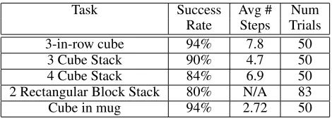
Task Success Avg # Num Rate Steps Trials
3-in-row cube 94% 7.8 50
3 Cube Stack 90% 4.7 50
4 Cube Stack 84% 6.9 50
2 Rectangular Block Stack 80% N/A 83
Cube in mug 94% 2.72 50
Table 2: Results from robot experiments.
estimate of the maximum. Here, we setη = 0.2Figure 5b shows the comparison. Notice that the average reward per episode is approximately 15% worse with the hierarchy as compared to without it. We conclude that while the value function hierarchy is sometimes needed to train in a reason-able period of time, it should be avoided if possible.
Robot experiments
We performed robot experiments to get a sense of the kinds of tasks that deictic image mapping can help solve. We used a UR5 equipped with a Robotiq two finger gripper, as shown in Figure 6a. In all experiments, objects were dumped ran-domly onto a table in ranran-domly selected positions within an
50×50cm region within the manipulator workspace. All end-to-end motions commanded by the agent were planned using TrajOpt (Schulman et al. 2013) with the final gripper pose constrained to be orthogonal to the table. All images were acquired using a depth sensor (Structure IO, the light blue device in Figure 6a,b) mounted to the gripper. At the beginning of each time step, because of camera calibration inaccuracies, the robot took images from four different po-sitions above the table and stitched them together to create a complete 2-D image. Then, the system selected and per-formed a pick or place action consisting of a single colli-sion free motion followed by an opening or closing motion of the gripper. In all experiments, the system was trained in completely in simulation using OpenRAVE (Diankov and Kuffner 2008) using a simulated setup nearly identical to the physical robot. Then, the policy learned in simulation was executed and evaluated on the real robot. We evalu-ated performance for the following five tasks. All tasks had sparse rewards: the agent received 0 reward everywhere ex-cept upon reaching the goal state.
Three-in-a-row cube arrangement: In this task, three cubes were dumped onto a table and then re-oriented manu-ally so that each block had a fixed orientation with respect to the robot. The system was trained using the same parameters as used in simulation, but using four curriculum stages start-ing with a 10cm step size and annealstart-ing down to a 1cm step size. The agent received +1 reward for achieving a three-in-a-row alignment within ten time steps and zero otherwise. As shown in the first row of Table 2, we obtain a 94% task success rate over 50 trials.
Stacking three cubes:This task is the same as three-in-a-row (above) except that the agent now received +1 reward for stacking the three cubes. We obtain a 90% task success rate (second row of Table 2).
Stacking four cubes:This task is the same as above except that the agent must now stack four cubes (Figure 6b). We obtain an 84% task success rate (third row of Table 2). Stacking two rectangular blocks:In this task, eight rect-angular blocks were dumped on the table (Figure 6c). The robot received +1 reward every time it stacked one block on to of another (Figure 6d). After every successful stack, the top block was removed from the table by the experimenter. Unlike the three cube stacking/arranging tasks above, the action space for this task included 16 possible orienta-tions (similar to the simulation experiments). The agent was trained using a seven stage curriculum and the value func-tion hierarchy with η = 0.1 that reduced the number of actions from 51.2k down to 8.32k. This task is interesting because the agent must learn to balance long blocks on top of small blocks as shown in Figure 6d. The average success rate for two-block stacking attempts was 80% (fourth row of Table 2).
Cube in mug:Finally, we evaluated our approach on a task where the robot must pick up a cube and drop it into a mug (Figure 6f). During robot testing, at the start of each episode, a random mug was chosen from the selection of eight mugs shown in Figure 6e and was randomly placed on the table in a upright position along with a block. Importantly, these were novel mugs in the sense that they were different from any of the six randomly re-scaled mugs used to train the sys-tem. The agent received a reward of -0.1 when it moved the mug and +1 when it solved the task within no more than 10 time steps. The average task success rate here was 94% (last row in Table 2).
These five robot experiments suggest that deictic image maps can be used to solve a variety of robotic manipulation problems related to pick and place. The stacking-four-cubes experiment demonstrates that the approach can solve prob-lems that involve several pick/place actions. The stacking-two-rectangular blocks experiments shows that the method can perform relatively precise placements. Finally, the cube-in-mug experiment shows that the method can be trained to solve tasks involving novel objects.
Analysis
It turns out that deictic image mapping is theoretically cor-rect in the sense that optimal policies for the abstract MDP found using DQN induce optimal policies for the original system. We use the MDP homomorphism framework. Definition 2 (MDP Homomorphism, Ravindran 2004 (Ravindran 2004)). An MDP homomorphism from an MDP M = hS,A, T, Ri onto M0 = hS0,A0, T0, R0i is
a tuple of mappings,hf,{gs|s ∈ S}i, wheref : S → S0
is a state mapping,gs : A → A0, s ∈ S is a set of action
mappings, and the following two conditions are satisfied for alls∈ S,a∈ A, ands0 ∈ S0:
T0(f(s), gs(a), s0) =
X
¯
s∈{s∈S|f(s)=s0}
T(s, a,s)¯ (5)
R0(f(s), gs(a)) = R(s, a). (6)
S0 andA0 are theabstractstate and action sets,
Equa-(a) (b) (c) (d) (e) (f)
Figure 6: (a) Experimental scenario. (b) four block stacking task. (c) initial block configuration for rectangular block stacking. (d) rectangular block stacking task. (d) Mugs used in cube-in-mug task. (f) Cube-in-mug task.
tion 2 encodes an actionain terms ofcrop(I, am). SinceI
is the image or signed distance function perceived by sen-sors, this is astate-dependent mapping. The MDP Homo-morphism framework is specifically relevant to this situation because, unlike other abstraction frameworks (Givan, Dean, and Greig 2003; Dean, Givan, and Leach 1997), it allows for state dependent action abstraction. If we can identify condi-tions under which the action mapping of Equation 2 in con-junction with the state mapping of Equation 3 is an MDP homomorphism, then a theorem exists that says that a solu-tion to the abstract MDP induces a solusolu-tion in the original problem:
Theorem 1 (Optimal value equivalence, Ravindran 2004 (Ravindran 2004)). LetM0 =hS0,A0, T0, R0ibe the
homomorphic image ofM=hS,A, T, Riunder the MDP homomorphism,hf,{gs|s ∈ S}i. For any(s, a)∈ S × A, Q∗(s, a) =Q0∗(f(s), gs(a)).
Here,Q∗(·)andQ0∗(·) denote the optimal action-value function for the underlying MDP and the abstract MDP re-spectively. We now show that the deictic image mapping in-duces an MDP homomorphism.
Theorem 2. Given a move-effect system with state set
S; action set A; transition function T such that for all
t ∈ R>0, θt+1 is conditionally independent of st given crop(It, am(t)); a deictic image mappinghf,{gs|s∈ S}i;
and an abstract reward functionR0 : S0× A0 →
R; then
there exist a reward function Rand an abstract transition functionT0for whichhf,{gs|s∈ S}iis an MDP
homomor-phism from M = hS,A, T, RitoM0 = hS0,A0, T0, R0i.
Proof. See Appendix 1 in supplementary materials.
As a consequence of Theorem 2 and 1, we know that op-timal solutions to the abstract MDP induced by Equations 3 and 2 induce optimal solutions to the original move-effect system as long as the conditions of Theorem 2 are satisfied.
Related Work, Limitations, and Discussion
This work is related to prior applications of deixis in AI. Evidence exists that the human brain leverages deictic rep-resentations during performance of motor tasks (Ballard et al. 1997). Whitehead and Ballard proposed an application of deixis to reinforcement learning, focusing on blocks world applications in particular (Whitehead and Ballard 1991).
While our representations are only loosely related to Bal-lard’s computational architecture, our work is closely related to the psychological evidence in (Ballard et al. 1997).
The analysis section of this paper leverages the MDP Homomorphism framework introduced by Ravindran and Barto (Ravindran 2004; Ravindran and Barto 2003). MDP Homomorphisms are related to other MDP abstraction meth-ods (Givan, Dean, and Greig 2003; Dean, Givan, and Leach 1997). However, unlike those methods, the MDP Homomor-phisms allow for the state-dependent action abstraction, a critical part of our proposed abstraction.
This paper is also generally related to a variety of recent works exploring deep learning for robotic manipulation. The work of (Zeng et al. 2018) is related to ours in that they estimate a Q-function over a large number of grasping and pushing actions, in their case by creating a fully convolu-tional Q-network. The work of (Li, Hsu, and Lee 2018) also involves a large action space of push actions, pruned us-ing a heuristic. Other pieces of recent related manipulation work are (Fang et al. 2018) and (Gualtieri, ten Pas, and Platt 2018) who each propose methods of learning task-relevant grasps in the context of a reinforcement learning problem. Our work can be loosely viewed as an extension of recent grasp detection work by (Mahler et al. 2017) and (Gualtieri et al. 2016), however the focus here is on more complex ma-nipulation tasks rather than just grasping.
In contrast to some of the work cited above, a nice aspect of our method is that it can be applied to a relatively gen-eral class of problems, such as those explored in our experi-ments. However, the method has important limitations. First, limits on the number of actions that can be realistically con-sidered on a given time step means that it will be important to find ways to limit the number of motion actions that need to be considered. Another limitation is that the deictic image patch used to represent a motion only “sees” a portion of the total image. As a result, our method is not well suited to re-spond to non-local state information. Although we have not yet tried this, we expect that this problem can be solved by using a “foveated” action patch that “sees” the world around a potential action choice at multiple resolutions.
Acknowledgements
References
Ballard, D. H.; Hayhoe, M. M.; Pook, P. K.; and Rao, R. P. 1997. Deictic codes for the embodiment of cognition. Be-havioral and Brain Sciences20(4):723–742.
Bengio, Y.; Louradour, J.; Collobert, R.; and Weston, J. 2009. Curriculum learning. InProceedings of the 26th an-nual international conference on machine learning, 41–48. ACM.
Blake, A., and Zisserman, A. 1987. Visual reconstruction. MIT press.
Dean, T.; Givan, R.; and Leach, S. 1997. Model reduction techniques for computing approximately optimal solutions for markov decision processes. InProceedings of the Thir-teenth conference on Uncertainty in artificial intelligence, 124–131. Morgan Kaufmann Publishers Inc.
Diankov, R., and Kuffner, J. 2008. Openrave: A planning ar-chitecture for autonomous robotics. Technical Report CMU-RI-TR-08-34, Robotics Institute, Pittsburgh, PA.
Fang, K.; Zhu, Y.; Garg, A.; Kurenkov, A.; Mehta, V.; Fei-Fei, L.; and Savarese, S. 2018. Learning task-oriented grasp-ing for tool manipulation from simulated self-supervision.
arXiv preprint arXiv:1806.09266.
Givan, R.; Dean, T.; and Greig, M. 2003. Equivalence no-tions and model minimization in markov decision processes.
Artificial Intelligence147(1-2):163–223.
Gualtieri, M., and Platt, R. 2018. Learning 6-DoF grasping and pick-place using attention focus. InProceedings of The 2nd Conference on Robot Learning, volume 87 of Proceed-ings of Machine Learning Research, 477–486. PMLR. Gualtieri, M.; ten Pas, A.; Saenko, K.; and Platt, R. 2016. High precision grasp pose detection in dense clutter. InIEEE Int’l Conf. on Intelligent Robots and Systems.
Gualtieri, M.; ten Pas, A.; and Platt, R. 2018. Pick and place without geometric object models. InIEEE Int’l Conf. on Robotics and Automation (ICRA). IEEE.
Li, J. K.; Hsu, D.; and Lee, W. S. 2018. Push-net: Deep pla-nar pushing for objects with unknown physical properties. InRobotics: Science and Systems (RSS).
Lillicrap, T. P.; Hunt, J. J.; Pritzel, A.; Heess, N.; Erez, T.; Tassa, Y.; Silver, D.; and Wierstra, D. 2015. Continuous control with deep reinforcement learning. arXiv preprint arXiv:1509.02971.
Mahler, J.; Liang, J.; Niyaz, S.; Laskey, M.; Doan, R.; Liu, X.; Ojea, J. A.; and Goldberg, K. 2017. Dex-net 2.0: Deep learning to plan robust grasps with synthetic point clouds and analytic grasp metrics. arXiv preprint arXiv:1703.09312.
Mnih, V.; Kavukcuoglu, K.; Silver, D.; Graves, A.; Antonoglou, I.; Wierstra, D.; and Riedmiller, M. 2013. Play-ing atari with deep reinforcement learnPlay-ing. arXiv preprint arXiv:1312.5602.
Ravindran, B., and Barto, A. 2003. Smdp homomorphisms: An algebraic approach to abstraction in semi markov deci-sion processes. InInternational Joint Conference on Artifi-cial Intelligence (IJCAI), 1011–1016.
Ravindran, B. 2004. An algebraic approach to abstraction in reinforcement learning. Ph.D. Dissertation, University of Massachusetts at Amherst.
Schaul, T.; Quan, J.; Antonoglou, I.; and Silver, D. 2015. Prioritized experience replay. arXiv preprint arXiv:1511.05952.
Schulman, J.; Ho, J.; Lee, A.; Awwal, I.; Bradlow, H.; and Abbeel, P. 2013. Finding locally optimal, collision-free tra-jectories with sequential convex optimization. InRobotics: Science and Systems. Citeseer.
Wang, Z.; Schaul, T.; Hessel, M.; Van Hasselt, H.; Lanc-tot, M.; and De Freitas, N. 2015. Dueling network ar-chitectures for deep reinforcement learning. arXiv preprint arXiv:1511.06581.
Whitehead, S. D., and Ballard, D. H. 1991. Learning to per-ceive and act by trial and error. Machine Learning7(1):45– 83.