Deep Hidden Physics Models:
Deep Learning of Nonlinear Partial Differential Equations
Maziar Raissi maziar [email protected]
Division of Applied Mathematics Brown University
Providence, RI, 02912, USA
Editor:Manfred Opper
Abstract
We put forth a deep learning approach for discovering nonlinear partial differential equa-tions from scattered and potentially noisy observaequa-tions in space and time. Specifically, we approximate the unknown solution as well as the nonlinear dynamics by two deep neu-ral networks. The first network acts as a prior on the unknown solution and essentially enables us to avoid numerical differentiations which are inherently ill-conditioned and un-stable. The second network represents the nonlinear dynamics and helps us distill the mechanisms that govern the evolution of a given spatiotemporal data-set. We test the effectiveness of our approach for several benchmark problems spanning a number of scien-tific domains and demonstrate how the proposed framework can help us accurately learn the underlying dynamics and forecast future states of the system. In particular, we study the Burgers’, Korteweg-de Vries (KdV), Kuramoto-Sivashinsky, nonlinear Schr¨odinger, and Navier-Stokes equations.
Keywords: Systems Identification, Data-driven Scientific Discovery, Physics Informed Machine Learning, Predictive Modeling, Nonlinear Dynamics, Big Data
1. Introduction
Recent advances in machine learning in addition to new data recordings and sensor technolo-gies have the potential to revolutionize our understanding of the physical world in modern application areas such as neuroscience, epidemiology, finance, and dynamic network analy-sis where first-principles derivations may be intractable (Rudy et al., 2017). In particular, many concepts from statistical learning can be integrated with classical methods in ap-plied mathematics to help us discover sufficiently sophisticated and accurate mathematical models of complex dynamical systems directly from data. This integration of nonlinear dy-namics and machine learning opens the door for principled methods for model construction, predictive modeling, nonlinear control, and reinforcement learning strategies. The literature on data-driven discovery of dynamical systems (Crutchfield and McNamara, 1987) is vast and encompasses equation-free modeling (Kevrekidis et al., 2003), artificial neural networks (Raissi et al., 2018a; Gonzalez-Garcia et al., 1998; Anderson et al., 1996; Rico-Martinez et al., 1992), nonlinear regression (Voss et al., 1999), empirical dynamic modeling (Sugi-hara et al., 2012; Ye et al., 2015), modeling emergent behavior (Roberts, 2014), automated inference of dynamics (Schmidt et al., 2011; Daniels and Nemenman, 2015a,b), normal form
c
identification in climate (Majda et al., 2009), nonlinear Laplacian spectral analysis (Gian-nakis and Majda, 2012), modeling emergent behavior (Roberts, 2014), Koopman analysis (Mezi´c, 2005; Budiˇsi´c et al., 2012; Mezi´c, 2013; Brunton et al., 2017), automated inference of dynamics (Schmidt et al., 2011; Daniels and Nemenman, 2015a,b), and symbolic regression (Bongard and Lipson, 2007; Schmidt and Lipson, 2009). More recently, sparsity (Tibshirani, 1996) has been used to determine the governing dynamical system (Brunton et al., 2016; Mangan et al., 2016; Wang et al., 2011; Schaeffer et al., 2013; Ozoli¸nˇs et al., 2013; Mackey et al., 2014; Brunton et al., 2014; Proctor et al., 2014; Bai et al., 2014; Tran and Ward, 2016).
Less well studied is how to discover closed form mathematical models of the physical world expressed by partial differential equations from scattered data collected in space and time. Inspired by recent developments inphysics-informed deep learning(Raissi et al., 2017c,d), we construct structured nonlinear regression models that can uncover the dynamic dependencies in a given set of spatio-temporal data, and return a closed form model that can be subsequently used to forecast future states. In contrast to recent approaches to systems identification (Brunton et al., 2016; Rudy et al., 2017), here we do not need to have direct access or approximations to temporal or spatial derivatives. Moreover, we are using a richer class of function approximators to represent the nonlinear dynamics and consequently we do not have to commit to a particular family of basis functions. Specifically, we consider nonlinear partial differential equations of the general form
ut=N(t, x, u, ux, uxx, . . .), (1)
where N is a nonlinear function of time t, space x, solution u and its derivatives.1 Here, the subscripts denote partial differentiation in either time t or space x.2 Given a set of scattered and potentially noisy observations of the solutionu, we are interested in learning the nonlinear function N and consequently identifying an infinite dimensional dynamical system (i.e., partial differential equation) that governs the evolution of the observed spatio-temporal data.
For instance, let us assume that we would like to discover the Burger’s equation (Bas-devant et al., 1986) in one space dimension ut=−uux+ 0.1uxx. Although not pursued in the current work, a viable approach (Rudy et al., 2017) to tackle this problem is to create a dictionary of possible terms and write the following expansion
N(t, x, u, ux, uxx, . . .) = α0,0+α1,0u+α2,0u2+α3,0u3+
α0,1ux+α1,1uux+α2,1u2ux+α3,1u3ux+ α0,2uxx+α1,2uuxx+α2,2u2uxx+α3,2u3uxx+ α0,3uxxx+α1,3uuxxx+α2,3u2uxxx+α3,3u3uxxx.
1. The solutionu = (u1, . . . , un) could be n dimensional in which case ux denotes the collection of all
element-wise first order derivatives ∂u1 ∂x, . . . ,
∂un
∂x. Similarly, uxxincludes all element-wise second order
derivatives ∂2u1 ∂x2 , . . . ,
∂2un
∂x2 .
2. The spacex= (x1, x2, . . . , xm) could be a vector of dimensionm. In this case,uxdenotes the collection
of all first order derivative ux1, ux2, . . . , uxm and uxxrepresents the set of all second order derivatives
Given the aforementioned large collection of candidate terms for constructing the partial differential equation, one could then use sparse regression techniques (Rudy et al., 2017) to determine the coefficients αi,j and consequently the right-hand-side terms that are con-tributing to the dynamics. A huge advantage of this approach is the interpretability of the learned equations. However, there are two major drawbacks associated with this method.
First, it relies on numerical differentiation to compute the derivatives involved in equa-tion (1). Derivatives are taken either using finite differences for clean data or with poly-nomial interpolation in the presence of noise. Numerical approximations of derivatives are inherently ill-conditioned and unstable (Baydin et al., 2015) even in the absence of noise in the data. This is due to the introduction of truncation and round-off errors inflicted by the limited precision of computations and the chosen value of the step size for finite differencing. Thus, this approach requires far more data points than library functions. This need for using a large number of points lies more in the numerical evaluation of derivatives than in supplying sufficient data for the regression.
Second, in applying the algorithm (Rudy et al., 2017) outlined above we assume that the chosen library is sufficiently rich to have a sparse representation of the time dynamics of the dataset. However, when applying this approach to a dataset where the dynamics are in fact unknown it is not unlikely that the basis chosen above is insufficient. Specially, in higher dimensions (i.e., for inputx or outputu) the required number of terms to include in the library increases exponentially. Moreover, an additional issue with this approach is that it can only estimate parameters appearing as coefficients. For example, this method can-not estimate parameters of a partial differential equation (e.g., the sine-Gordon equation) involving a term like sin(αu(x)) with α being the unknown parameter, even if we include sines and cosines in the dictionary of possible terms.
One could avoid the first drawback concerning numerical differentiation by assigning prior distributions in the forms of Gaussian processes (Raissi et al., 2017b; Raissi and Kar-niadakis, 2017; Raissi et al., 2017a, 2018b) or neural networks (Raissi et al., 2017c,d) to the unknown solution u. Derivatives of the prior on u can now be evaluated at machine pre-cision using symbolic or automatic differentiation (Baydin et al., 2015). This removes the requirement for having or generating data on derivatives of the solutionu. This is enabling as it allows us to work with noisy observations of the solution u, scattered in space and time. Moreover, this approach requires far fewer data points than the method proposed in (Rudy et al., 2017) simply because, as explained above, the need for using a large number of data points was due to the numerical evaluation of derivatives. The choice to place a prior on the unknown solution u is motivated by modern techniques for solving forward and inverse problems involving partial differential equations, where the unknown solution is approximated either by a neural network (Raissi et al., 2017c,d; Raissi, 2018; Raissi et al., 2018a) or a Gaussian process (Raissi et al., 2018b; Raissi and Karniadakis, 2017; Raissi et al., 2017a,b; Raissi, 2017; Perdikaris et al., 2017; Raissi and Karniadakis, 2016).
N by a deep neural network is the novelty of the current work. Deep neural networks are a richer family of function approximators and consequently we do not have to commit to a particular class of basis functions such as polynomials or sines and cosines. This expressive-ness comes at the cost of losing interpretability of the learned dynamics. However, there is nothing hindering the use of a particular class of basis functions in order obtain more interpretable equations (Raissi et al., 2017d).
2. Solution methodology
We proceed by approximating both the solutionu and the nonlinear function N with two deep neural networks3 and define a deep hidden physics model f to be given by
f :=ut− N(t, x, u, ux, uxx, . . .). (2)
We obtain the derivatives of the neural network u with respect to time t and space x by applying the chain rule for differentiating compositions of functions using automatic dif-ferentiation (Baydin et al., 2015). It is worth emphasizing that automatic difdif-ferentiation is different from, and in several aspects superior to, numerical or symbolic differentiation; two commonly encountered techniques of computing derivatives. Numerical differentiation entails the finite difference approximation of derivatives using values of the original function evaluated at some sample points. Due to the introduction of truncation and round-off er-rors inflicted by the limited precision of computations and the chosen value of the step size for finite differencing, numerical approximations of derivatives are inherently ill-conditioned and unstable (Baydin et al., 2015). Symbolic differentiation uses expression manipulation in computer algebra systems such as Mathematica, Maxima, and Maple. Symbolic meth-ods require models to be defined as closed-form expressions, ruling out or severely limiting algorithmic control flow and expressivity (Baydin et al., 2015).
Without proper introduction, one might assume that automatic differentiation is either a type of numerical or symbolic differentiation (Baydin et al., 2015). Confusion can arise because automatic differentiation does in fact provide numerical values of derivatives (as opposed to derivative expressions) and it does so by using symbolic rules of differentiation (but keeping track of derivative values as opposed to the resulting expressions), giving it a two-sided nature that is partly symbolic and partly numerical (Baydin et al., 2015). In its most basic description (Baydin et al., 2015), automatic differentiation relies on the fact that all numerical computations are ultimately compositions of a finite set of elementary operations for which derivatives are known. Combining the derivatives of the constituent operations through the chain rule gives the derivative of the overall composition. This allows accurate evaluation of derivatives at machine precision with ideal asymptotic efficiency and only a small constant factor of overhead. In particular, to compute the derivatives involved in equation (2) we rely on Tensorflow (Abadi et al., 2016) which is a popular and relatively well documented open source software library for automatic differentiation and deep learn-ing computations. In TensorFlow, before a model is run, its computational graph is defined
statically rather than dynamically as for instance in PyTorch (Paszke et al., 2017). This is an important feature as it allows us to create and compile the entire computational graph for a deep hidden physics model (2) only once and keep it fixed throughout the training procedure. This leads to significant reduction in the computational cost of the proposed framework.
Parameters of the neural networks u and N can be learned by minimizing the sum of squared errors loss function
SSE := N
X
i=1
|u(ti, xi)−ui|2+|f(ti, xi)|2
, (3)
where{ti, xi, ui}Ni=1 denote the training data on u. The term|u(ti, xi)−ui|2 tries to fit the data by adjusting the parameters of the neural networku while the term|f(ti, xi)|2 learns the parameters of the networkN by trying to satisfy the partial differential equation (1) at the collocation points (ti, xi). Training the parameters of the neural networks uand N can be performed simultaneously by minimizing the sum of squared error (3) or in a sequential fashion by training ufirst and N second.
How can we make sure that the algorithm presented above results in an acceptable functionN? One answer would be to solve the learned equations and compare the result-ing solution to the solution of the exact partial differential equation. However, it should be pointed out that the learned function N is a black-box function; i.e., we do not know its functional form. Consequently, none of the classical partial differential equation solvers such as finite differences, finite elements or spectral methods are applicable here. Therefore, to solve the learned equations we have no other choice than to resort to modern black-box solvers such asphysic informed neural networks(PINNs) introduced in (Raissi et al., 2017c). The steps involved in PINNs as solvers4 are similar to equations (1), (2), and (3) with the nonlinear functionN being known and the data residing on the boundary of the domain.
In the following, to keep the paper self-contained, we briefly explain the PINNs algorithm (Raissi et al., 2017c) for solving non-linear partial differential equations in as few sentences as possible. The PINNs algorithm is very general and for a more detailed exposure we refer the interested reader to (Raissi et al., 2017c). However, for pedagogical purposes, we explain the algorithm by applying it to the problem of solving the Burgers’ equation (see section 3.1) as an example accompanied by periodic boundary conditions; i.e.,
ut+uux−0.1uxx= 0, x∈[−8,8], u(0, x) =−sin(πx/8),
u(t,−8) =u(t,8), ux(t,−8) =ux(t,8).
We approximate the unknown solution u(t, x) to the Burgers’ equation by a deep neural network. Consequently, the corresponding physic informed neural network (PINN) takes
the form
f :=ut+uux−0.1uxx.
To be precise, for the cases studied in the current work, the physic informed neural network f(t, x) has a form similar tof :=N(u, ux, uxx) for some pre-trained (see equation 3) neural network N with its parameters being kept fixed. We acquire the required derivatives to compute the residual networkf by applying the chain rule for differentiating compositions of functions using automatic differentiation (Baydin et al., 2015). The shared parameters between the neural networks u(t, x) and f(t, x) can be learned by minimizing the mean squared errors loss function
M SE=M SE0+M SEb+M SEf, where
M SE0 = N10 PNi=10 |u(0, xi0)−ui0|2,
M SEb = N1b PNi=1b |u(tib,−8)−u(tib,8)|2+|ux(tib,−8)−ux(tib,8)|2
,
M SEf = N1f PNi=1f |f(tif, xif)|2. Here, {xi0, hi0}N0
i=1 denote the initial data generated in this example by the initial function
−sin(πx/8), {tib}Nb
i=1 correspond to the collocation points on the boundary, and{tif, xif} Nf
i=1 represents the collocation points on the residual networkf(t, x). Consequently,M SE0 cor-responds to the loss on the initial data, M SEb enforces the periodic boundary conditions, andM SEf penalizes the Burgers’ equation for not being satisfied on the collocation points. This example encapsulates all of the important ingredients of the PINNs algorithm (Raissi et al., 2017c) and can be straightforwardly generalized to arbitrary partial differential equa-tions where the boundary condiequa-tions should be treated on a case by case basis (see Raissi et al., 2017c).
3. Results
The proposed framework provides a universal treatment of nonlinear partial differential equations of fundamentally different nature. This generality will be demonstrated by ap-plying the algorithm to a wide range of canonical problems spanning a number of scientific domains including the Burgers’, Korteweg-de Vries (KdV), Kuramoto-Sivashinsky, non-linear Schr¨odinger, and Navier-Stokes equations. These examples are motivated by the pioneering work of Rudy et al. (2017). All data and codes used in this manuscript are publicly available on GitHub at https://github.com/maziarraissi/DeepHPMs.
3.1 Burgers’ equation
Let us start with the Burgers’ equation arising in various areas of engineering and applied mathematics, including fluid mechanics, nonlinear acoustics, gas dynamics, and traffic flow (Basdevant et al., 1986). In one space dimension, the Burgers’ equation reads as
To obtain a set of training and test data, we simulate the Burger’s equation (4) using conventional spectral methods. Specifically, starting from an initial condition u(0, x) =
−sin(πx/8), x∈[−8,8] and assuming periodic boundary conditions, we integrate equation (4) up to the final time t = 10. We use the Chebfun package (Driscoll et al., 2014) with a spectral Fourier discretization with 256 modes and a fourth-order explicit Runge-Kutta temporal integrator with time-step size 10−4. The solution is saved every ∆t= 0.05 to give us a total of 201 snapshots. Out of this data-set, we generate a smaller training subset, scattered in space and time, by randomly sub-sampling 10000 data points from time t= 0 tot= 6.7. We call the portion of the domain from timet= 0 tot= 6.7 the training portion. The rest of the domain from timet= 6.7 to the final timet= 10 will be referred to as the test portion. Using this terminology, we are in fact sub-sampling from the original dataset only in the training portion of the domain. Given the training data, we are interested in learning N as a function of the solution uand its derivatives up to the 2nd order5; i.e.,
ut=N(u, ux, uxx). (5)
We represent the solution u by a 5-layer deep neural network with 50 neurons per hidden layer. Furthermore, we let N to be a neural network with 2 hidden layers and 100 neurons per hidden layer. As for the activation functions, we use sin(x). In general, the choice of a neural network’s architecture (e.g., number of layers/neurons and form of activation functions) is crucial and in many cases still remains an art that relies on one’s ability to bal-ance the trade off betweenexpressivity andtrainability of the neural network (Raghu et al., 2016). Our empirical findings so far indicate that deeper and wider networks are usually more expressive (i.e., they can capture a larger class of functions) but are often more costly to train (i.e., a feed-forward evaluation of the neural network takes more time and the opti-mizer requires more iterations to converge). Moreover, the sinusoid (i.e., sin(x)) activation function seems to be numerically more stable than tanh(x), at least while computing the residual neural network f (see equation 2). However, these observations should be inter-preted as conjectures rather than as firm results6. In this work, we have tried to choose the neural networks’ architectures in a consistent fashion throughout the manuscript. Conse-quently, there might exist other architectures that improve some of the results reported in the current work.
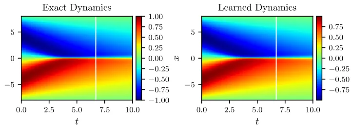
The neural networksu andN are trained by minimizing the sum of squared errors loss of equation (3). To illustrate the effectiveness of our approach, we solve the learned partial differential equation (5), along with periodic boundary conditions and the same initial con-dition as the one used to generate the original dataset, using the PINNs algorithm (Raissi et al., 2017c). The original dataset alongside the resulting solution of the learned partial differential equation are depicted in figure 1. This figure indicates that our algorithm is able to accurately identify the underlying partial differential equation with a relativeL2-error of 4.78e-03. It should be highlighted that the training data are collected in roughly two-thirds of the domain between times t= 0 and t= 6.7. The algorithm is thus extrapolating from
5. A detailed study of the choice of the order will be provided later in this section.
0.0 2.5 5.0 7.5 10.0 t
−5 0 5
x
Exact Dynamics
−1.00
−0.75
−0.50
−0.25 0.00 0.25 0.50 0.75 1.00
0.0 2.5 5.0 7.5 10.0 t
−5 0 5
x
Learned Dynamics
−0.75
−0.50
−0.25 0.00 0.25 0.50 0.75
Figure 1: Burgers equation: A solution to the Burger’s equation (left panel) is compared to the corresponding solution of the learned partial differential equation (right panel). The identified system correctly captures the form of the dynamics and accurately reproduces the solution with a relativeL2-error of 4.78e-03. It should be emphasized that the training data are collected in roughly two-thirds of the domain between times t= 0 and t= 6.7 represented by the white vertical lines. The algorithm is thus extrapolating from time t = 6.7 onwards. The relative L2-error on the training portion of the domain is 3.89e-03.
Clean data 1% noise 2% noise 5% noise Relative L2-error 4.78e-03 2.64e-02 1.09e-01 4.56e-01
Table 1: Burgers’ equation: Relative L2-error between solutions of the Burgers’ equation and the learned partial differential equation as a function of noise corruption level in the data. Here, the total number of training data as well as the neural network architectures are kept fixed.
0.0 2.5 5.0 7.5 10.0
t −5
0 5
x
Exact Dynamics
0.0 0.2 0.4 0.6 0.8 1.0
0.0 2.5 5.0 7.5 10.0
t −5
0 5
x
Learned Dynamics
0.0 0.2 0.4 0.6 0.8 1.0
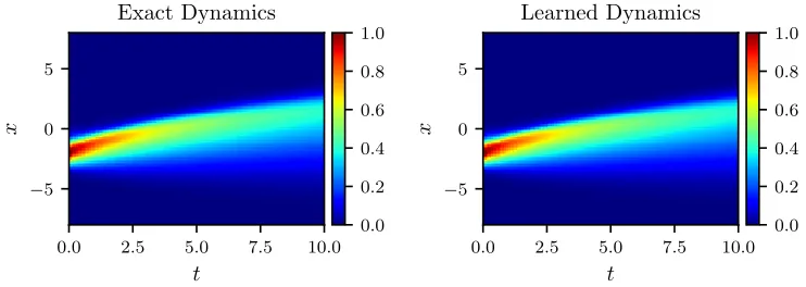
Figure 2: Burgers equation: A solution to the Burger’s equation (left panel) is compared to the corresponding solution of the learned partial differential equation (right panel). The identified system correctly captures the form of the dynamics and accurately reproduces the solution with a relativeL2-error of 3.44e-02. It should be highlighted that the algorithm is trained on a dataset totally different from the one used in this figure.
mandating further investigations. For instance, how common techniques such as batch nor-malization, drop out, andL1/L2 regularization (Goodfellow et al., 2016) could enhance the robustness of the proposed algorithm with respect to the neural network architectures as well as noise in the data.
0.0 2.5 5.0 7.5 10.0 t
−5 0 5
x
Exact Dynamics
−1.00
−0.75
−0.50
−0.25 0.00 0.25 0.50 0.75 1.00
0.0 2.5 5.0 7.5 10.0 t
−5 0 5
x
Learned Dynamics
−0.75
−0.50
−0.25 0.00 0.25 0.50 0.75
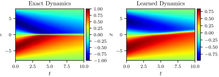
Figure 3: Burgers equation: A solution to the Burger’s equation (left panel) is compared to the corresponding solution of the learned partial differential equation (right panel). The algorithm fails to generalize to the new test data. The relativeL2 -error between the exact and the learned solutions is equal to 2.99e-01. Here, we are training on the dataset presented in figure 2 and testing on the one depicted in figure 1. In other words, we are swapping the roles of these two datasets. This observation suggests that the dynamics (see figure 1) generated by −sin(πx/8) as the initial condition is a reacher one compared to the dynamics (see figure 2) generated by exp(−(x+ 2)2). This is also evident from a visual comparison of the two datasets given in figures 1 and 2.
Moreover, if we make the nonlinear functionN both time and space dependent the relative L2-error increases even further to 1.46e+00. A possible explanation for this behavior could be that some of the dynamics in the training data is now being explained by time t or space x. This makes the algorithm over-fit to the training data and consequently harder for it to generalize to datasets it has never seen before. Based on our experience more data seems to help resolve this issue. Another interesting observation is that if we train on the dataset presented in figure 2 and test on the one depicted in figure 1, i.e., swap the roles of these two datasets, the algorithm fails to generalize to the new test data. To be precise, as depicted in figure 3, the relativeL2-error between the exact and the learned solutions is now equal to 2.99e-01. This observation suggests that the dynamics (see figure 1) generated by
−sin(πx/8) as the initial condition is a richer one compared to the dynamics (see figure 2) generated by exp(−(x+ 2)2). This is also evident from a visual comparison of the datasets given in figures 1 and 2.
1st order 2nd order 3rd order 4th order Relative L2-error 1.14e+00 1.29e-02 3.42e-02 5.54e-02
Table 2: Burgers’ equation: Relative L2-error between solutions of the Burgers’ equation and the learned partial differential equation as a function of the highest order of spatial derivatives included in our formulation. For instance, the case correspond-ing to the 3rd order means that we are lookcorrespond-ing for a nonlinear function N such that ut =N(u, ux, uxx, uxxx). Here, the total number of training data as well as the neural network architectures are kept fixed and the data are assumed to be noiseless.
assuming period boundary conditions. Consequently, in cases of practical interest, the available information on the boundary of the domain could help us determine the order of the partial differential equation we are try to identify. With this in mind, let us study the robustness of our framework with respect to the highest order of the derivatives in-cluded in equation (5). As for the boundary conditions, we use u(t,−8) = u(t,8) and ux(t,−8) = ux(t,8) when solving the identified partial differential equation regardless of the initial choice of its order. The results are summarized in table 2. The first column of table 2 demonstrates that a single first order derivative is clearly not enough to capture the second order dynamics of the Burgers’ equation. Moreover, the method seems to be gener-ally robust with respect to the number and order of derivatives included in the nonlinear function N. Therefore, in addition to any information residing on the domain boundary, studies such as table 2, albeit for training or validation datasets, could help us choose the best order for the underlying partial differential equation. In this case, table 2 suggests the order of the equation to be two.
In addition, it must be stated that including higher order derivatives comes at the cost of reducing the speed of the algorithm due to the growth in the complexity of the resulting computational graph for the corresponding deep hidden physics model (see equation 2). Also, another drawback is that higher order derivatives are usually less accurate specially if one uses single precision floating-point system (float32) rather than double precision (float64). It is true that automatic differentiation enables us to evaluate derivatives at machine precision, however, for float32 the machine epsilon is approximately 1.19e-07. For improved performance in terms of speed of the algorithm and constrained by usual GPU (graphics processing unit) platforms we often end up using float32 which boils down to committing an error of approximately 1.19e-07 while computing the required derivatives. The aforementioned issues do not seem to be too serious since computer infrastructure (both hardware and software) for deep learning is constantly improving.
3.2 The KdV equation
As a mathematical model of waves on shallow water surfaces one could consider the Korteweg-de Vries (KdV) equation. The KdV equation reads as
0 10 20 30 40 t
−20
−10 0 10 20
x
Exact Dynamics
−1.0
−0.5 0.0 0.5 1.0 1.5 2.0
0 10 20 30 40
t −20
−10 0 10 20
x
Learned Dynamics
−0.5 0.0 0.5 1.0 1.5 2.0
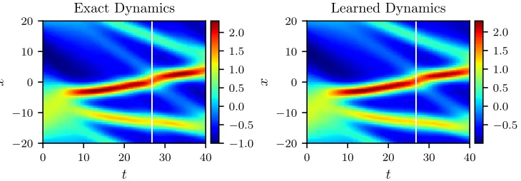
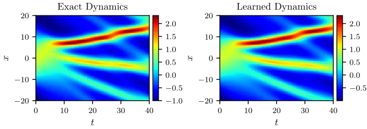
Figure 4: The KdV equation: A solution to the KdV equation (left panel) is compared to the corresponding solution of the learned partial differential equation (right panel). The identified system correctly captures the form of the dynamics and accurately reproduces the solution with a relativeL2-error of 6.28e-02. It should be emphasized that the training data are collected in roughly two-thirds of the domain between timest= 0 and t= 26.8 represented by the white vertical lines. The algorithm is thus extrapolating from time t = 26.8 onwards. The relative L2-error on the training portion of the domain is 3.78e-02.
To obtain a set of training data we simulate the KdV equation (6) using conventional spec-tral methods. In particular, we start from an initial condition u(0, x) =−sin(πx/20), x∈
[−20,20] and assume periodic boundary conditions. We integrate equation (6) up to the final timet= 40. We use the Chebfun package (Driscoll et al., 2014) with a spectral Fourier discretization with 512 modes and a fourth-order explicit Runge-Kutta temporal integrator with time-step size 10−4. The solution is saved every ∆t = 0.2 to give us a total of 201 snapshots. Out of this data-set, we generate a smaller training subset, scattered in space and time, by randomly sub-sampling 10000 data points from time t = 0 to t = 26.8. In other words, we are sub-sampling from the original dataset only in the training portion of the domain from time t = 0 to t = 26.8. Given the training data, we are interested in learning N as a function of the solution uand its derivatives up to the 3rd order7; i.e.,
ut=N(u, ux, uxx, uxxx). (7)
We represent the solution u by a 5-layer deep neural network with 50 neurons per hidden layer. Furthermore, we let N to be a neural network with 2 hidden layers and 100 neurons per hidden layer. As for the activation functions, we use sin(x). These two networks are trained by minimizing the sum of squared errors loss of equation (3). To illustrate the effectiveness of our approach, we solve the learned partial differential equation (7) using the PINNs algorithm (Raissi et al., 2017c). We assume periodic boundary conditions and the same initial condition as the one used to generate the original dataset. The resulting solution of the learned partial differential equation as well as the exact solution of the KdV equation are depicted in figure 4. This figure indicates that our algorithm is capable of accurately identifying the underlying partial differential equation with a relativeL2-error of
0 10 20 30 40 t
−20
−10 0 10 20
x
Exact Dynamics
−1.0
−0.5 0.0 0.5 1.0 1.5 2.0
0 10 20 30 40
t −20
−10 0 10 20
x
Learned Dynamics
−0.5 0.0 0.5 1.0 1.5 2.0
Figure 5: The KdV equation: A solution to the KdV equation (left panel) is compared to the corresponding solution of the learned partial differential equation (right panel). The identified system correctly captures the form of the dynamics and accurately reproduces the solution with a relativeL2-error of 3.44e-02. It should be highlighted that the algorithm is trained on a dataset different from the one shown in this figure.
6.28e-02. It should be highlighted that the training data are collected in roughly two-thirds of the domain between times t= 0 and t= 26.8. The algorithm is thus extrapolating from time t= 26.8 onwards. The corresponding relative L2-error on the training portion of the domain is 3.78e-02.
To test the algorithm even further, let us change the initial condition to cos(−πx/20) and solve the KdV equation (6) using the conventional spectral method outlined above. We compare the resulting solution to the one obtained by solving the learned partial differential equation (5) using the PINNs algorithm (Raissi et al., 2017c). It is worth emphasizing that the algorithm is trained on the dataset depicted in figure 4 and is being tested on a different dataset as shown in figure 5. The surprising result reported in figure 5 strongly indicates that the algorithm is accurately learning the underlying partial differential equation; i.e., the nonlinear function N. The algorithm hasn’t seen the dataset shown in figure 5 during model training and is yet capable of achieving a relatively accurate approximation of the true solution. To be precise, the identified system reproduces the solution to the KdV equation with a relative L2-error of 3.44e-02.
3.3 Kuramoto-Sivashinsky equation
As a canonical model of a pattern forming system with spatio-temporal chaotic behavior we consider the Sivashinsky equation. In one space dimension the Kuramoto-Sivashinsky equation reads as
ut=−uux−uxx−uxxxx. (8)
0 20 40
t −10
−5 0 5 10
x
Exact Dynamics
−3
−2
−1 0 1 2 3
0 20 40
t −10
−5 0 5 10
x
Learned Dynamics
−2
−1 0 1 2 3
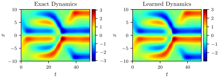
Figure 6: Kuramoto-Sivashinsky equation: A solution to the Kuramoto-Sivashinsky equa-tion (left panel) is compared to the corresponding soluequa-tion of the learned partial differential equation (right panel). The identified system correctly captures the form of the dynamics and reproduces the solution with a relative L2-error of 7.63e-02.
[−10,10] and integrate equation (8) up to the final time t= 50. We employ the Chebfun package (Driscoll et al., 2014) with a spectral Fourier discretization with 512 modes and a fourth-order explicit Runge-Kutta temporal integrator with time-step size 10−5. The snap-shots are saved every ∆t = 0.2. From this dataset, we create a smaller training subset, scattered in space and time, by randomly sub-sampling 10000 data points from time t= 0 to the final timet = 50.0. Given the resulting training data, we are interested in learning
N as a function of the solution u and its derivatives up to the 4rd order8; i.e.,
ut=N(u, ux, uxx, uxxx, uxxxx). (9)
We let the solutionuto be represented by a 5-layer deep neural network with 50 neurons per hidden layer. Furthermore, we approximate the nonlinear function N by a neural network with 2 hidden layers and 100 neurons per hidden layer. As for the activation functions, we use sin(x). These two networks are trained by minimizing the sum of squared errors loss of equation (3). To demonstrate the effectiveness of our approach, we solve the learned partial differential equation (9) using the PINNs algorithm (Raissi et al., 2017c). We assume the same initial and boundary conditions as the ones used to generate the original dataset. The resulting solution of the learned partial differential equation alongside the exact solution of the Kuramoto-Sivashinsky equation are depicted in figure 6. This figure indicates that our algorithm is capable of identifying the underlying partial differential equation with a relative L2-error of 7.63e-02. Here and in the rest of the current manuscript, the test and training datasets appear to be the same. However, it should be emphasized that during test time the only pieces of information given to the PINNs algorithm are the initial and boundary data in addition to the learned functionN. This means that results such as figure 6 are sufficient to clearly communicate the message that the algorithm has approximately learned the correct equations. Moreover, whether a particular dataset is rich enough so that
0 25 50 75 100
t
0 25 50 75 100
x
Exact Dynamics
−3
−2
−1 0 1 2 3
0 25 50 75 100
t
0 25 50 75 100
x
Learned Dynamics
−2
−1 0 1 2
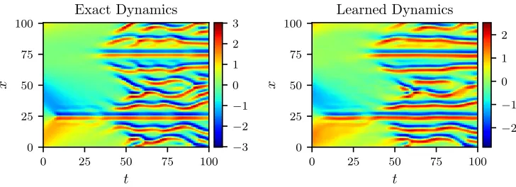
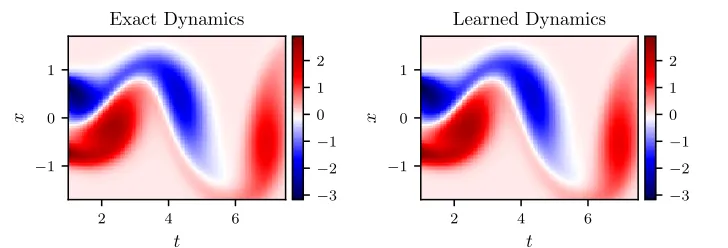
Figure 7: Kuramoto-Sivashinsky equation: A solution to the Kuramoto-Sivashinsky equa-tion is depicted in the left panel. The corresponding soluequa-tion of the learned partial differential equation is shown in the right panel. This problem remains stubbornly unsolved in the face of the algorithm proposed in the current work. In fact, the identified system reproduces the solution with a relative L2-error of 4.17e-01, which is unsatisfactorily large.
the algorithm generalizes to other datasets generated by different initial conditions is a fun-damentally different question which has been extensively studied so far in the manuscript using the Burgers’ and KdV examples.
solvers for partial differential equations is still in its infancy and more collaborative work is needed to set the foundations in this field.
3.4 Nonlinear Schr¨odinger equation
The one-dimensional nonlinear Schr¨odinger equation is a classical field equation that is used to study nonlinear wave propagation in optical fibers and/or waveguides, Bose-Einstein con-densates, and plasma waves. This example aims to highlight the ability of our framework to handle complex-valued solutions as well as different types of nonlinearities in the governing partial differential equations. The nonlinear Schr¨odinger equation is given by
ψt= 0.5iψxx+i|ψ|2ψ. (10) Letu denote the real part ofψ andv the imaginary part. Then, the nonlinear Schr¨odinger equation can be equivalently written as a system of partial differential equations
ut=−0.5vxx−(u2+v2)v,
vt= 0.5uxx+ (u2+v2)u. (11) In order to assess the performance of our method, we simulate equation (10) using con-ventional spectral methods to create a high-resolution data set. Specifically, starting from an initial state ψ(0, x) = 2 sech(x) and assuming periodic boundary conditions ψ(t,−5) = ψ(t,5) and ψx(t,−5) = ψx(t,5), we integrate equation (10) up to a final time t = π/2 using the Chebfun package (Driscoll et al., 2014). We are in fact using a spectral Fourier discretization with 512 modes and a fourth-order explicit Runge-Kutta temporal integrator with time-step ∆t=π/2·10−6. The solution is saved approximately every ∆t= 0.0031 to give us a total of 501 snapshots. Out of this data-set, we generate a smaller training subset, scattered in space and time, by randomly sub-sampling 10000 data points from time t= 0 up to the final timet=π/2. Given the resulting training data, we are interested in learning two nonlinear functions N1 and N2 as functions of the solutions u, v and their derivatives up to the 2nd order9; i.e.,
ut=N1(u, v, ux, vx, uxx, vxx),
vt=N2(u, v, ux, vx, uxx, vxx). (12) We represent the solutionsuandvby two 5-layer deep neural networks with 50 neurons per hidden layer. Furthermore, we letN1andN2to be two neural networks with 2 hidden layers and 100 neurons per hidden layer. As for the activation functions, we use sin(x). These four networks are trained by minimizing a sum of squared errors loss function similar to equation (3). To illustrate the effectiveness of our approach, we solve the learned partial differential equation (12), along with periodic boundary conditions and the same initial condition as the one used to generate the original dataset, using the PINNs algorithm (Raissi et al., 2017c). The original dataset (in absolute values, i.e.,|ψ|=√u2+v2) alongside the resulting solution (also in absolute values) of the learned partial differential equation are depicted in figure 8. This figure indicates that our algorithm is able to accurately identify the underlying partial differential equation with a relative L2-error of 6.28e-03.
0.0 0.5 1.0 1.5
t −4
−2 0 2 4
x
Exact Dynamics
0.5 1.0 1.5 2.0 2.5 3.0 3.5
0.0 0.5 1.0 1.5
t −4
−2 0 2 4
x
Learned Dynamics
0.5 1.0 1.5 2.0 2.5 3.0 3.5 4.0
Figure 8: Nonlinear Schr¨odinger equation: Absolute value of a solution to the nonlinear Schr¨odinger equation (left panel) is compared to the absolute value of the corre-sponding solution of the learned partial differential equation (right panel). The identified system correctly captures the form of the dynamics and accurately re-produces the absolute value of the solution with a relativeL2-error of 6.28e-03.
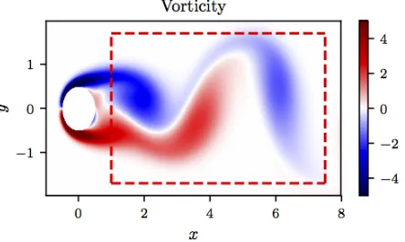
Figure 9: Navier-Stokes equation: A snapshot of the vorticity field of a solution to the Navier-Stokes equations for the fluid flow past a cylinder. The dashed red box in this panel specifies the sampling region.
3.5 Navier-Stokes equation
Let us consider the Navier-Stokes equation in two dimensions10 (2D) given explicitly by wt=−uwx−vwy+ 0.01(wxx+wyy), (13)
where w denotes the vorticity, u the x-component of the velocity field, and v the y -component. To generate a training dataset for this problem we follow the exact same instructions as the ones provided in (Kutz et al., 2016; Rudy et al., 2017). Specifically,
2 4 6 t −1
0 1
x
Exact Dynamics
−3
−2
−1 0 1 2
2 4 6
t −1
0 1
x
Learned Dynamics
−3
−2
−1 0 1 2
Figure 10: Navier-Stokes equation: A randomly picked snapshot of a solution to the Navier-Stokes equation (left panel) is compared to the corresponding snapshot of the solution of the learned partial differential equation (right panel). The identified system correctly captures the form of the dynamics and accurately reproduces the solution with a relativeL2-error of 5.79e-03 in space and time.
we simulate the Navier-Stokes equations describing the two-dimensional fluid flow past a circular cylinder at Reynolds number 100 using the Immersed Boundary Projection Method (Taira and Colonius, 2007; Colonius and Taira, 2008). This approach utilizes a multi-domain scheme with four nested domains, each successive grid being twice as large as the previous one. Length and time are nondimensionalized so that the cylinder has unit diameter and the flow has unit velocity. Data is collected on the finest domain with dimensions 9×4 at a grid resolution of 449×199. The flow solver uses a 3rd-order Runge Kutta integration scheme with a time step of ∆t = 0.02, which has been verified to yield well-resolved and converged flow fields. After simulation converges to steady periodic vortex shedding, 151 flow snapshots are saved every ∆t= 0.02. We use a small portion of the resulting data-set for model training. In particular, we subsample 50000 data points, scattered in space and time, in the rectangular region (dashed red box) downstream of the cylinder as shown in figure 9.
Given the training data, we are interested in learningN as a function of the stream-wise uand transversev velocity components in addition to the vorticitywand its derivatives up to the 2nd order11; i.e.,
wt=N(u, v, w, wx, wxx). (14)
We represent the solutionwby a 5-layer deep neural network with 200 neurons per hidden layer. Furthermore, we let N to be a neural network with 2 hidden layers and 100 neurons per hidden layer. As for the activation functions, we use sin(x). These two networks are trained by minimizing the sum of squared errors loss
SSE:= N
X
i=1
|w(ti, xi, yi)−wi|2+|f(ti, xi, yi)|2
,
where{ti, xi, ui, vi, wi}N
i=1 denote the training data on u and f(ti, xi, yi) is given by f(ti, xi, yi) :=wt(ti, xi, yi)− N(ui, vi, w(ti, xi, yi), wx(ti, xi, yi), wxx(ti, xi, yi)).
To illustrate the effectiveness of our approach, we solve the learned partial differential equation (14), in the region specified in figure 9 by the dashed red box, using the PINNs algorithm (Raissi et al., 2017c). We use the exact solution to provide us with the required Dirichlet boundary conditions as well as the initial condition needed to solve the learned partial differential equation (14). A randomly picked snapshot of the vorticity field in the original dataset alongside the corresponding snapshot of the solution of the learned partial differential equation are depicted in figure 10. This figure indicates that our algorithm is able to accurately identify the underlying partial differential equation with a relative L2-error of 5.79e-03 in space and time.
4. Summary and Discussion
We have presented a deep learning approach for extracting nonlinear partial differential equations from spatio-temporal datasets. The proposed algorithm leverages recent devel-opments in automatic differentiation to construct efficient algorithms for learning infinite dimensional dynamical systems using deep neural networks. In order to validate the per-formance of our approach we had no other choice than to rely on black-box solvers (see Raissi et al., 2017c). This signifies the importance of developing general purpose partial differential equation solvers. Developing these types of solvers is still in its infancy and more collaborative work is needed to bring them to the maturity level of conventional methods such as finite elements, finite differences, and spectral methods which have been around for more than half a century or so.
There exist a series of open questions mandating further investigations. For instance, many real-world partial differential equations depend on parameters and, when the pa-rameters are varied, they may go through bifurcations (e.g., the Reynold number for the Navier-Stokes equations). Here, the goal would be to collect data from the underlying dynamics corresponding to various parameter values, and infer the parameterized partial differential equation. Another exciting avenue of future research would be to apply convolu-tional architectures (Goodfellow et al., 2016) for mitigating the complexity associated with partial differential equations with very high-dimensional inputs. These types of equations appear routinely in dynamic programming, optimal control, or reinforcement learning. We envision that the proposed framework, as outlined in the current work, can be straightfor-wardly extended to such high-dimensional cases. Early evidence of this claim can be found in (Raissi, 2018), where the author devises an algorithm that is scalable to high-dimensions and is capable of circumventing the tyranny of numerical discretization. In addition, the approach advocated in the current work is also highly scalable to the big data regimes encountered while studying such high-dimensional cases simply because the data can be processed in mini-batches.
handful of them do not take this form, including the Boussinesq type equationutt−uxx− 2α(uux)x−βuxxtt = 0. It would be interesting to extend the framework outlined in the current work to incorporate all such cases. In addition, it would be an exciting continuation of the current work to extend the proposed methodology to stochastic partial differential equations. In fact, independent realizations of the underlying noise process (e.g., Brownian motion) could act as training data (Raissi, 2018). In the end, it is not always clear what measurements of a dynamical system to take. Even if we did know, collecting these mea-surements might be prohibitively expensive. It is well-known that time-delay coordinates of a single variable can act as additional variables. It might be interesting to investigate this idea for the infinite dimensional setting of partial differential equations. In terms of applications, it would be intriguing to see how the proposed framework would perform on Geostationary Operational Environmental Satellites (GOES) data (e.g., sea surface tem-perature data) which could be retrieved fromhttps://podaac.jpl.nasa.gov/.
Acknowledgments
This work received support by the DARPA EQUiPS grant N66001-15-2-4055 and the AFOSR grant FA9550-17-1-0013. All data and codes used in this manuscript are publicly available on GitHub at https://github.com/maziarraissi/DeepHPMs.
References
Mart´ın Abadi, Ashish Agarwal, Paul Barham, Eugene Brevdo, Zhifeng Chen, Craig Citro, Greg S Corrado, Andy Davis, Jeffrey Dean, Matthieu Devin, et al. Tensorflow: Large-scale machine learning on heterogeneous distributed systems.arXiv preprint arXiv:1603.04467, 2016.
JS Anderson, IG Kevrekidis, and R Rico-Martinez. A comparison of recurrent training algorithms for time series analysis and system identification. Computers & chemical engineering, 20:S751–S756, 1996.
Zhe Bai, Thakshila Wimalajeewa, Zachary Berger, Guannan Wang, Mark Glauser, and Pramod K Varshney. Low-dimensional approach for reconstruction of airfoil data via compressive sensing. AIAA Journal, 2014.
Cea Basdevant, M Deville, P Haldenwang, JM Lacroix, J Ouazzani, R Peyret, Paolo Or-landi, and AT Patera. Spectral and finite difference solutions of the Burgers equation. Computers & fluids, 14(1):23–41, 1986.
Atilim Gunes Baydin, Barak A Pearlmutter, Alexey Andreyevich Radul, and Jeffrey Mark Siskind. Automatic differentiation in machine learning: a survey. arXiv preprint arXiv:1502.05767, 2015.
Steven L Brunton, Jonathan H Tu, Ido Bright, and J Nathan Kutz. Compressive sensing and low-rank libraries for classification of bifurcation regimes in nonlinear dynamical systems. SIAM Journal on Applied Dynamical Systems, 13(4):1716–1732, 2014.
Steven L Brunton, Joshua L Proctor, and J Nathan Kutz. Discovering governing equations from data by sparse identification of nonlinear dynamical systems. Proceedings of the National Academy of Sciences, 113(15):3932–3937, 2016.
Steven L Brunton, Bingni W Brunton, Joshua L Proctor, Eurika Kaiser, and J Nathan Kutz. Chaos as an intermittently forced linear system. Nature Communications, 8, 2017.
Marko Budiˇsi´c, Ryan Mohr, and Igor Mezi´c. Applied koopmanism a. Chaos: An Interdis-ciplinary Journal of Nonlinear Science, 22(4):047510, 2012.
Tim Colonius and Kunihiko Taira. A fast immersed boundary method using a nullspace approach and multi-domain far-field boundary conditions. Computer Methods in Applied Mechanics and Engineering, 197(25):2131–2146, 2008.
James P Crutchfield and Bruce S McNamara. Equations of motion from a data series. Complex systems, 1(417-452):121, 1987.
Bryan C Daniels and Ilya Nemenman. Automated adaptive inference of phenomenological dynamical models. Nature communications, 6, 2015a.
Bryan C Daniels and Ilya Nemenman. Efficient inference of parsimonious phenomenological models of cellular dynamics using s-systems and alternating regression. PloS one, 10(3): e0119821, 2015b.
Tobin A Driscoll, Nicholas Hale, and Lloyd N Trefethen. Chebfun guide, 2014.
Dimitrios Giannakis and Andrew J Majda. Nonlinear laplacian spectral analysis for time series with intermittency and low-frequency variability. Proceedings of the National Academy of Sciences, 109(7):2222–2227, 2012.
R Gonzalez-Garcia, R Rico-Martinez, and IG Kevrekidis. Identification of distributed pa-rameter systems: A neural net based approach. Computers & chemical engineering, 22: S965–S968, 1998.
Ian Goodfellow, Yoshua Bengio, and Aaron Courville. Deep learning. MIT press, 2016.
Ioannis G Kevrekidis, C William Gear, James M Hyman, Panagiotis G Kevrekidid, Olof Runborg, Constantinos Theodoropoulos, et al. Equation-free, coarse-grained multiscale computation: Enabling mocroscopic simulators to perform system-level analysis. Com-munications in Mathematical Sciences, 1(4):715–762, 2003.
J Nathan Kutz, Steven L Brunton, Bingni W Brunton, and Joshua L Proctor. Dynamic Mode Decomposition: Data-Driven Modeling of Complex Systems, volume 149. SIAM, 2016.
Andrew J Majda, Christian Franzke, and Daan Crommelin. Normal forms for reduced stochastic climate models. Proceedings of the National Academy of Sciences, 106(10): 3649–3653, 2009.
Niall M Mangan, Steven L Brunton, Joshua L Proctor, and J Nathan Kutz. Inferring biological networks by sparse identification of nonlinear dynamics. IEEE Transactions on Molecular, Biological and Multi-Scale Communications, 2(1):52–63, 2016.
Igor Mezi´c. Spectral properties of dynamical systems, model reduction and decompositions. Nonlinear Dynamics, 41(1):309–325, 2005.
Igor Mezi´c. Analysis of fluid flows via spectral properties of the koopman operator. Annual Review of Fluid Mechanics, 45:357–378, 2013.
Vidvuds Ozoli¸nˇs, Rongjie Lai, Russel Caflisch, and Stanley Osher. Compressed modes for variational problems in mathematics and physics. Proceedings of the National Academy of Sciences, 110(46):18368–18373, 2013.
Adam Paszke, Sam Gross, Soumith Chintala, Gregory Chanan, Edward Yang, Zachary DeVito, Zeming Lin, Alban Desmaison, Luca Antiga, and Adam Lerer. Automatic dif-ferentiation in pytorch. 2017.
Paris Perdikaris, Maziar Raissi, Andreas Damianou, ND Lawrence, and George Em Karni-adakis. Nonlinear information fusion algorithms for data-efficient multi-fidelity modelling. Proc. R. Soc. A, 473(2198):20160751, 2017.
Joshua L Proctor, Steven L Brunton, Bingni W Brunton, and JN Kutz. Exploiting spar-sity and equation-free architectures in complex systems. The European Physical Journal Special Topics, 223(13):2665–2684, 2014.
M. Raghu, B. Poole, J. Kleinberg, S. Ganguli, and J. Sohl-Dickstein. On the expressive power of deep neural networks. arXiv preprint arXiv:1606.05336, 2016.
Maziar Raissi. Parametric gaussian process regression for big data. arXiv preprint arXiv:1704.03144, 2017.
Maziar Raissi. Forward-backward stochastic neural networks: Deep learning of high-dimensional partial differential equations. arXiv preprint arXiv:1804.07010, 2018.
Maziar Raissi and George Karniadakis. Deep multi-fidelity Gaussian processes. arXiv preprint arXiv:1604.07484, 2016.
Maziar Raissi and George Em Karniadakis. Hidden physics models: Machine learning of nonlinear partial differential equations. Journal of Computational Physics, 2017.
Maziar Raissi, Paris Perdikaris, and George Em Karniadakis. Machine learning of linear differential equations using Gaussian processes. Journal of Computational Physics, 348: 683 – 693, 2017b. ISSN 0021-9991. doi: http://dx.doi.org/10.1016/j.jcp.2017.07.050. URLhttp://www.sciencedirect.com/science/article/pii/S0021999117305582.
Maziar Raissi, Paris Perdikaris, and George Em Karniadakis. Physics informed deep learn-ing (part i): Data-driven solutions of nonlinear partial differential equations. arXiv preprint arXiv:1711.10561, 2017c.
Maziar Raissi, Paris Perdikaris, and George Em Karniadakis. Physics informed deep learn-ing (part ii): Data-driven discovery of nonlinear partial differential equations. arXiv preprint arXiv:1711.10566, 2017d.
Maziar Raissi, Paris Perdikaris, and George Em Karniadakis. Multistep neural networks for data-driven discovery of nonlinear dynamical systems. arXiv preprint arXiv:1801.01236, 2018a.
Maziar Raissi, Paris Perdikaris, and George Em Karniadakis. Numerical gaussian pro-cesses for time-dependent and nonlinear partial differential equations. SIAM Journal on Scientific Computing, 40(1):A172–A198, 2018b.
R Rico-Martinez, K Krischer, IG Kevrekidis, MC Kube, and JL Hudson. Discrete-vs. continuous-time nonlinear signal processing of cu electrodissolution data. Chemical En-gineering Communications, 118(1):25–48, 1992.
Anthony John Roberts. Model emergent dynamics in complex systems. SIAM, 2014.
Samuel H. Rudy, Steven L. Brunton, Joshua L. Proctor, and J. Nathan Kutz. Data-driven discovery of partial differential equations. Science Advances, 3(4), 2017. doi: 10.1126/ sciadv.1602614. URL http://advances.sciencemag.org/content/3/4/e1602614.
Hayden Schaeffer, Russel Caflisch, Cory D Hauck, and Stanley Osher. Sparse dynamics for partial differential equations. Proceedings of the National Academy of Sciences, 110(17): 6634–6639, 2013.
Michael Schmidt and Hod Lipson. Distilling free-form natural laws from experimental data. science, 324(5923):81–85, 2009.
Michael D Schmidt, Ravishankar R Vallabhajosyula, Jerry W Jenkins, Jonathan E Hood, Abhishek S Soni, John P Wikswo, and Hod Lipson. Automated refinement and inference of analytical models for metabolic networks. Physical biology, 8(5):055011, 2011.
George Sugihara, Robert May, Hao Ye, Chih-hao Hsieh, Ethan Deyle, Michael Fogarty, and Stephan Munch. Detecting causality in complex ecosystems. science, 338(6106):496–500, 2012.
Robert Tibshirani. Regression shrinkage and selection via the lasso. Journal of the Royal Statistical Society. Series B (Methodological), pages 267–288, 1996.
Giang Tran and Rachel Ward. Exact recovery of chaotic systems from highly corrupted data. arXiv preprint arXiv:1607.01067, 2016.
Henning U Voss, Paul Kolodner, Markus Abel, and J¨urgen Kurths. Amplitude equations from spatiotemporal binary-fluid convection data. Physical review letters, 83(17):3422, 1999.
Wen-Xu Wang, Rui Yang, Ying-Cheng Lai, Vassilios Kovanis, and Celso Grebogi. Predicting catastrophes in nonlinear dynamical systems by compressive sensing. Physical Review Letters, 106(15):154101, 2011.