COMPRESSIVE SPECTRAL RENORMALIZATION METHOD

(1)

C. BAYINDIR1,§

Abstract. In this paper a novel numerical scheme for finding the sparse self-localized states of a nonlinear system of equations with missing spectral data is introduced. As in the Petviashivili’s and the spectral renormalization method, the governing equation is transformed into Fourier domain, but the iterations are performed for far fewer number of spectral components (M) than classical versions of the these methods with higher number of spectral components (N). After the converge criteria is achieved forM components,

N component signal is reconstructed fromM components by using thel1 minimization technique of the compressive sampling. This method can be named as compressive spectral renormalization (CSRM) method. The main advantage of the CSRM is that, it is capable of finding the sparse self-localized states of the evolution equation(s) with many spectral data missing.

Keywords: Spectral renormalization, Petviashivili’s method, compressive sampling, spec-tral methods, nonlinear Schr¨odinger equation.

AMS Subject Classification: 81Q05, 65T50

1. Introduction

Missing spectral data in many branches of physics limits the applicability of analysis tools and devices and assessment techniques. These branches include but are not limited to optics, geophysics, electromagnetics and communication technology [1, 2]. Although shorter wavelengths are more vulnerable to attenuation compared to longer wavelengths, longer wavelengths can also be lost during their propagation in medium therefore any spectral component of a signal may be lost [3]. Different approaches are proposed to deal with problems that occur due to missing spectral data. Few of these approaches can be summarized as below: A modification of the singular spectrum analysis that analyzes time series with missing data is proposed in [1]. The missing data recovery via a nonparametric iterative adaptive approach and nonparametric spectral analysis with missing data via the expectation maximization algorithms are two other tools used in literature to overcome this problem [2]. The method of Marquardt is applied to a single 26-parameter equation, which models known long-wavelength loss mechanisms for rapid and accurate modeling of the spectral-loss profiles of lightguide fibers, in [4]. A compressive sensing (CS) based

1

Associate Professor, Engineering Faculty, I¸sık University, 34980, S¸ile, ˙Istanbul. Adjunct Professor, Engineering Faculty, Bo˘gazi¸ci University, 34342, Bebek, ˙Istanbul. e-mail: [email protected]; ORCID: http://orcid.org/0000-0002-3654-0469. § Manuscript received; January 22, 2017; accepted: September 9, 2018.

(2)

approach for stationary and non-stationary stochastic process power spectrum estimation with missing data is recently proposed in [5].

It remains an open question what the stable self-localized solutions would be in a non-linear field with missing spectral data. To overcome this problem, we propose a novel numerical scheme that can attain the stable sparse self-localized solutions of the nonlin-ear system of equations with many missing spectral data. We test the applicability of the

proposed method on a 1D Schr¨odinger-like equation which is widely used as a model

equa-tion in optics, hydrodynamics, quantum mechanics, Bose-Einstein condensaequa-tion [6, 7, 8]. The proposed method utilizes iterations in the Fourier domain for a far fewer number of

spectral components (M) than classical versions of the Petviashivili’s method or spectral

renormalization method (SRM) with higher number of spectral components (N). After

the converge criteria is achieved forM components, the signal with N components can be

reconstructed from M components by the l1 minimization technique of the compressive

sampling. The name proposed for this method is compressive spectral renormalization (CSRM) method. Compared to SRM, the main advantage of the CSRM is that, it is ca-pable of finding the sparse self-localized states of the evolution equation(s) with far fewer spectral data. For example for fiber optical communications, where some data is lost during the propagation of the optical pulse or considering memory and time constraints they may be intentionally ignored, CSRM can be used to find self localized states of the system of equations studied. We discuss the implementation of the proposed method and its advantages and limitations using single and dual soliton solutions of the NLS and an NLS-like equation with a potential used to model the photorefractive lattice solitons and with saturable nonlinearity.

2. Methodology

2.1. Review of the Spectral Renormalization Method. Self-localized solutions of many nonlinear systems can be found by various computational techniques such as

shoot-ing, self-consistency and relaxation [6]. Another method known is the Petviashvili’s

method which is based on transforming the governing nonlinear equation into Fourier space, as in the case of general Fourier spectral schemes [9, 10, 11, 12, 13, 14, 15, 16, 17, 18, 19, 20, 21, 22], and determining a convergence factor according to the degree of a single nonlinear term [6, 23]. This method was introduced by Petviashvili and applied to Kadomtsev-Petviashvili (2D Korteweg Vries) equation [23]. Later, it has been de-veloped and applied to many other systems which model many different phenomena such as lattice vortices, dark and gray solitons [6, 24]. Since Petviashvili’s method works well for nonlinearities with fixed homogeneity only, a novel spectral renormalization method (SRM) is proposed in [6, 25] which is capable of finding the localized solutions in waveg-uides with different types of nonlinearities. The SRM essentially transforms the governing equation into Fourier space and couples it to a nonlinear integral equation which is basically an energy conservation principle for the iterations in the Fourier space [6]. This coupling makes the initial conditions to converge to the self-localized solutions of the nonlinear system studied [6]. Also, some alternative methods, such as the pseudo-spectral method is proposed in order to find convergence factor explicitly from the governing equation, not by using the nonlinear integral equation [26, 27].

SRM is spectrally efficient, it can be applied to many different physical problems with different higher-order nonlinearities and is easy to implement [6]. Following [6], we give a brief review of the SRM considering a 1D NLS-like equation as

(3)

where z is the propagation direction of optical pulse, x is the transverse coordinate, i

denotes the imaginary number and ζ is complex amplitude of the optical field [6]. Using

the ansatz,ζ(x, z) =η(x, µ)exp(iµz), whereµ shows the soliton eigenvalue, the NLS-like

equation becomes

−µη+ηxx−V(x)η+N(|η|2)η= 0 (2)

Furthermore the 1D Fourier transform ofη can be obtained by

b

η(k) =F[η(x)] = Z +∞

−∞

η(x) exp[i(kx)]dx (3)

For a zero optical potential,V = 0, the 1D Fourier transform of Eq. (2) yields

b

η(k) =

FhN(|η|2η)i

µ+|k|2 (4)

This formula may be applied iteratively to find the self-localized solutions of the system studied, as first proposed by Petviashvili in [23]. However iterations of Eq. (3) may grow unboundedly or may tend to zero [6]. As proposed in [6], this problem can be solved by

introducing a new variable in the form η(x) = αξ(x) which has a 1D Fourier transform

b

η(k) =αξb(k). With these substitutions, Eq. (4) becomes

b

ξ(k) =

F

h

N(|α|2|ξ|2)ξ

i

µ+|k|2 =Rα[ξb(k)] (5)

and thus the iteration scheme is given as

b

ξj+1(k) =

FhN(|α_j|2|ξ_j|2)ξj i

µ+|k|2 (6)

For the normalization part of the SRM, an algebraic condition on the parameterαcan be

obtained using the energy conservation principle. Multiplying both sides of Eq. (5) with

the complex conjugate ofξb(k), which isξb∗(k), and integrating to evaluate the total energy,

the algebraic condition becomes

Z +∞ −∞

ξb(k)

2 dk=

Z +∞ −∞

b

ξ∗(k)Rα[ξb(k)]dk (7)

which is the normalization constraint that ensures the scheme to converge to a stable self-localized state, solitons. The procedure of obtaining self-self-localized solutions of a nonlinear system by the coupled equation analysis reviewed and summarized above is known as the spectral renormalization method (SRM) [6]. Starting with an initial condition in the form of a single or multi-Gaussians, Eq. (4) is applied to find the profile for next iteration step, then the normalization constraint given by Eq. (7) is applied. Iterations can be continued

until the convergence ofαis achieved.

Nonzero potentials (V 6= 0) are widely accepted as models for various optical media

such as nondefected or defected photonic crystals. Adding and substracting a pη term

with p > 0 from Eq. (2) in order to avoid singularity of the scheme [6], the 1D Fourier transform of Eq. (2) becomes

b

η(k) =(p+|µ|)ηb

p+|k|2 −

F[V η]−FhN(|η|2)ηi

p+|k|2 (8)

(4)

the 1D versions of the photorefractive solitons first reported in [28], we set the optical

potential as V = Iocos2(x) and the nonlinear term as N(|η|2) = −1/(1 +|η|2). As

before, one can define a new parameter η(x) = αξ(x) and evaluate its Fourier transform

as_bη(k) =αξb(k). With these substitutions iteration formula reads

b

ξj+1(k) =

(p+|µ|)

p+|k|2 ξbj −

F[V ξj]

p+|k|2

+ 1

p+|k|2F

"

ξj

1 +|αj|2|ξj|2

#

=Rαj[ξbj(k)]

(9)

The algebraic condition of the SRM for nonzero potential case can be attained by

mul-tiplying both sides of Eq. (9) with the complex conjugate of ξb(k), which is ξb∗(k), and

integrating to evaluate the total energy the normalization constraint becomes

Z +∞ −∞

ξb(k)

2 dk=

Z +∞ −∞

b

ξ∗(k)Rα[ξb(k)]dk (10)

As in the case of zero potentials, an initial condition in the form of a single or multi-Gaussians converges to self-localized states of the model equation when Eq. (9) is applied to find the profile for next iteration step and then the normalization constraint given

by Eq. (10) is applied. Iterations can be continued until the convergence of α with a

specified upper bound is achieved. A detailed discussion and application of SRM to 2D and second-harmonic generation problems can be seen in [6].

2.2. Review of the Compressive Sampling. Compressive sampling (CS) is an efficient sampling technique which exploits the sparsity of the signal for its reconstruction by using far fewer samples than the requirements of the Shannon-Nyquist sampling theorem [29, 30]. Since its introduction to the scientific community, CS has been intensively studied as a mathematical tool in applied mathematics and physics and currently sampling in various engineering devices such as the single pixel video cameras and efficient A-D converters is performed using CS. We give a very brief summary of the CS in this section and refer the reader to [29, 30] for a comprehensive analysis.

Letζ be aK-sparse signal withN elements. This means that onlyKof theN elements

ofζ are nonzero. Using orthonormal basis transformations with transformation a matrix

Ψ, ζ can be represented in transformed domain in terms of the basis functions. Typical

orthogonal transformations used in the literature include but are not limited to Fourier, wavelet or discrete cosine transforms (DCT). Using the orthogonal transformation it is

possible to express the signal asζ =Ψζbwhereζbis the coefficient vector. Discarding the

zero coefficients and keeping the non-zero coefficients ofζ, one can obtainζs=Ψζb_swhere

ζs denotes the signal with non-zero entries.

CS algorithm states that a K-sparse signal ζ which has N elements can exactly be

reconstructed fromM ≥Cµ2(Φ,Ψ)K log (N) measurements with a very high probability.

In hereC is a positive constant andµ2(Φ,Ψ) is the mutual coherence between the sensing

Φand transform basesΨ[29, 30]. Taking M projections randomly and using the sensing

matrixΦthe sampled signal can be written asg=Φζ. Therefore the CS problem can be

rewritten as min ζb l1

under constraint g=ΦΨζb (11)

where ζb l1 = P i ζbi

. Therefore among all signals that satisfy the given constraints

(5)

only one of the tools that can be used for finding the solution of this optimization problem. The sparse signals can also be recovered using other optimization techniques such as the

re-weightedl1 minimization or greedy pursuit algorithms [29, 30]. Details of the CS can

be seen in [29, 30].

2.3. Proposed Compressive Spectral Renormalization Method. In a classical SRM

letN be the number of the spectral components used to represent a self-localized solution

of an evolution equation(s). First we select M spectral components at random, where

M < N, and apply SRM for those M components. The random selection of the number

M needs to be done carefully depending on width of theK-sparse self-localized state since

M needs to satisfy theM =O(Klog(N/K)) condition of the CS. Starting from the initial

conditions, iterations are performed for obtaining the convergent self-localized states for

M components. After the converge criteria is achieved forM components, N component

signal is reconstructed fromM components by using thel1 minimization technique of the

CS. This method can be named as compressive spectral renormalization (CSRM) method. The advantage of the CSRM is that, it is capable of finding the sparse self-localized states

of the evolution equation(s) withN −M spectral data missing. In practice, for example

in a typical photonic crystal, only few of the spectral data would be expected to be lost, if any, during the propagation of the optical pulse. In that case, CSRM would be used to find the self-localized states of the system with the same accuracy of the SRM. Also one can intentionally undersample the sparse optical signal with monochromators are only used for selected components, but the accurate self-localized state can still be reconstructed using CSRM using only those selected components. It is possible to make the selection

of M components deterministically as well, but in that case CS solution would produce

some replicated patterns in the solution which need to be filtered in that case [31]. A similar procedure based on CS which exploits the sparsity of the simulated signal is proposed for general spectral schemes in [31, 32, 33, 34]. In these works, the main advantage of using CS in a spectral scheme is to improve the numerical simulation time and computer memory requirements of the sparse signals. CSRM can also be computationally

advantageous depending on how largeN−M is and the number of iteration steps needed

to obtain a convergent solution but for a more general SRM this advantage would be more

clear. If the ansatzζ(x, z) =η(x, µ)exp(iµ(z)z), whereµ(z) shows a propagation distance

dependent soliton eigenvalue, would be used, then finding the self-localized state at any

z would be necessary and thus CSRM would also be computationally very advantageous

while there is negligible accuracy difference between CSRM and SRM.

Although sparsity property of the self-localized states of the model NLS-like equation

in the physical domain is used and random selection ofM components are done in Fourier

space, for a state which is sparse in Fourier domain random samples can be taken in the physical domain and the CSRM can be applied in a pseudospectral manner. Additionally the CSRM method can be extended to other spectral methods, such as wavelets, DCTs, Chebyshev and Legendre polynomials, just to name a few.

3. Results and Discussion

3.1. Single and Dual Soliton Solutions of the NLS Equation for Zero Optical Potential. It is well known that NLS equation, which can be obtained by settingV = 0

andN(|ζ|2) =|ζ|2 in Eq. (1), admits single and dual humped soliton solutions in the form

of sech functions. In this section we assess the accuracy and advantages of the proposed CSRM using these single and dual soliton solutions. The parameters of the computations

(6)

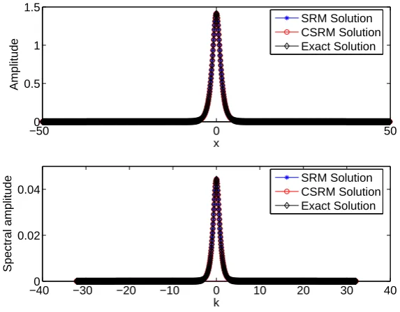
In Figure 1, the N = 1024 component SRM and M = 256 component CSRM are compared with the exact single soliton solution of the NLS equation. The initial condition

for this simulation is simply a Gaussian in the form of exp (−x2_{). The convergence is}

defined as the normalized change of α is less than 10−15. Both the SRM and CSRM

converge to the exact single sech type soliton solution within few iteration steps. Both of the SRM and CSRM are in excellent agreement with the exact solution as it can be seen in the figure. The normalized root-mean-square error calculated using the exact single sech

type solution and CSRM solution is 7.74×10−5 in the physical domain and is 7.70×10−5

in the Fourier domain. The two methods are in excellent agreement as it can be seen in Figure 1 while CSRM is more advantageous against missing spectral data since it uses

onlyM = 256 components.

−500 0 50

0.5 1 1.5

x

Amplitude

SRM Solution CSRM Solution Exact Solution

−400 −30 −20 −10 0 10 20 30 40

0.02 0.04

k

Spectral amplitude

Figure 1. Comparison of exact, N = 1024 component SRM and M = 256 component CSRM solutions for a) single soliton b) their spectra

In Figure 2, theN = 512 component SRM andM = 64 component CSRM are compared

with the exact single soliton solution of the NLS equation. The initial condition for this simulation is again a Gaussian. As before, the convergence is defined as the normalized

change of α to be less than 10−15 and both the SRM and CSRM converge to the exact

single sech type soliton solution within few iteration steps. Both of the SRM and CSRM are in good agreement with the exact solution as shown in figure. The normalized root-mean-square error for this case, which is calculated using the exact single sech type solution

and CSRM solution, is 1.42×10−2 in the physical domain and is 2.00×10−2 in the Fourier

domain. Compared to the results of the previous case depicted in Figure 1, error slightly

increases due to increased undersampling ratio (N/M). The two methods are in good

agreement as it can be seen in Figure 2 while CSRM is again more advantageous and

robust against missing spectral data than the SRM since it uses onlyM = 64 components

for the reconstruction of the self-localized state in the form of single soliton.

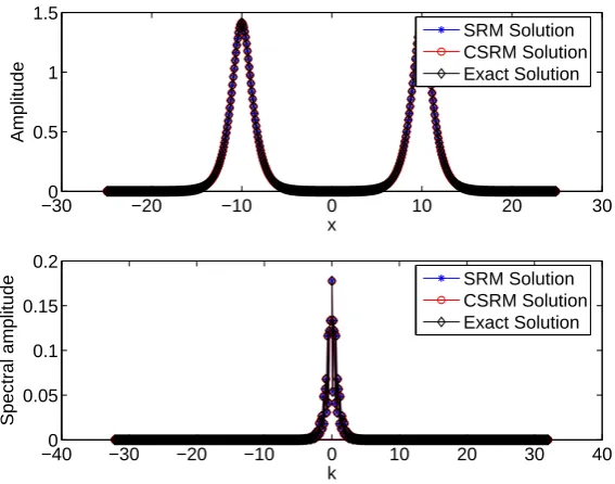
N = 512 component SRM andM = 128 component CSRM are compared with the dual

soliton solution of the NLS in Figure 3. The initial condition for this simulation is simply

(7)

−500 0 50 0.5

1 1.5

x

Amplitude

−200 −15 −10 −5 0 5 10 15 20

0.02 0.04

k

Spectral amplitude

Figure 2. Comparison of exact, N = 512 component SRM and M = 64 com-ponent CSRM solutions for a) single soliton b) their spectra

−300 −20 −10 0 10 20 30

0.5 1 1.5

x

Amplitude

−400 −30 −20 −10 0 10 20 30 40

0.05 0.1 0.15 0.2

k

Spectral amplitude

Figure 3. Comparison of exact,N = 512 component SRM andM = 128 com-ponent CSRM solutions for a) dual soliton b) their spectra

−x0=x1 = 10. The convergence for dual soliton simulations is defined as the normalized

change of α to be less than 10−5, since a smaller error bound may lead to single soliton

solution. Both the SRM and CSRM converges to the exact dual sech type soliton solution within few iteration steps. Both of the methods are in excellent agreement as it can be seen in the figure. The normalized root-mean-square error calculated using the exact single

(8)

in the Fourier domain. Compared to the case with same N and M depicted in Figure 1, the slight increase in the error is due to dual soliton profile is wider than single soliton profile, thus has less zero entries which starts to violate the sparsity condition of the CS.

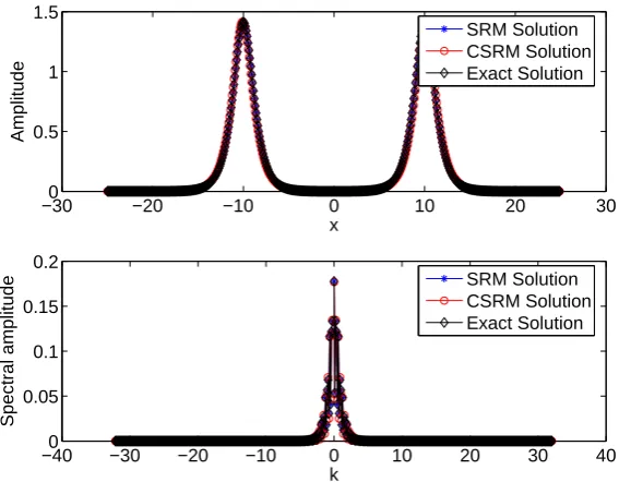
We compare the N = 512 component SRM and the M = 64 component CSRM with

the exact dual soliton solution of the NLS in Figure 4. The initial condition for this

simulation is again superposition of two Gaussians with unit amplitudes located at −10

and 10. As before, the upper bound for the convergence criteria ofα is selected as 10−5.

Both the SRM and CSRM converges to the exact dual sech type soliton solution within few iteration steps. For this case, the normalized root-mean-square error calculated using the

exact dual sech type soliton solution and CSRM solution is 1.32×10−2in physical domain

and 4.60×10−3 in the Fourier domain. The two methods are in acceptable agreement

as it can be seen in the figure. Compared to the case with same N and M depicted in

Figure 3, the increase in the error is due to the dual soliton profile that has less zero values compared to single soliton, which causes the sparsity condition of the CS to be violated. It is natural to expect that with higher undersampling ratios (i.e. more missing spectral data), the error will increase and CSRM may eventually fail. However the capability of CSRM to capture self-localized solutions despite these large undersampling ratios shows that it can be a very useful method in evaluating self-localized solutions in many systems with missing spectral data.

−300 −20 −10 0 10 20 30

0.5 1 1.5

x

Amplitude

−400 −30 −20 −10 0 10 20 30 40

0.05 0.1 0.15 0.2

k

Spectral amplitude

Figure 4. Comparison of exact, N = 512 component SRM and M = 64 com-ponent CSRM solutions for a) dual solitons b) their spectra

3.2. Single and Dual Soliton Solutions of NLS-like Equation for Nonzero Op-tical Potential. Turning our attention to the NLS-like equation given in Eq. (1) for a

nonzero optical potential of V = Iocos2(x) and the nonlinear term given as N(|η|2) =

−1/(1 +|η|2) which are used in practice [28], the iteration formula becomes Eq. (9). In

this iteration formula the parameters are selected asI0 = 1, p= 10, µ= 0.8.

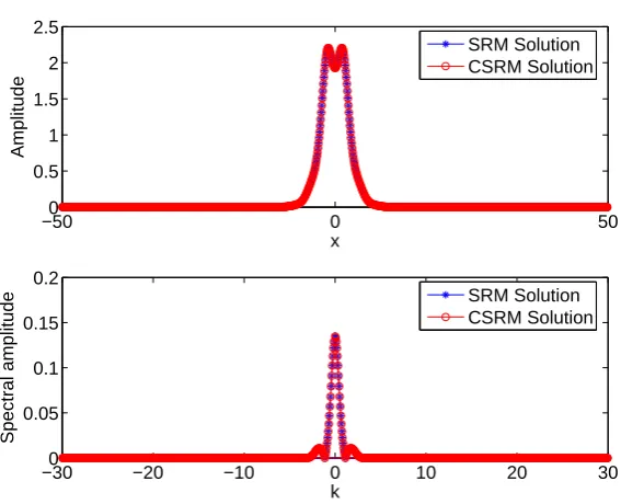
In Figure 5, N = 512 component SRM and M = 128 component CSRM solutions are

(9)

in the form of exp (−x2_{). The convergence is defined as the normalized change of} _α_{to be}

less than 10−15_{. Both the SRM and CSRM converge to the solution shown in Figure 5}

within few iteration steps. The SRM and CSRM solutions are in excellent agreement as one can see in the figure. The normalized root-mean-square difference calculated using the

SRM solution and CSRM solution is 2.47×10−4 in the physical domain and is 1.14×10−4

in the Fourier domain. The accuracy difference is of negligible importance but the CSRM

is more advantageous and robust against missing spectral data since it uses onlyM = 128

components for the reconstruction of the single soliton solution.

−500 0 50

0.5 1 1.5 2 2.5

x

Amplitude

SRM Solution CSRM Solution

−15 −10 −5 0 5 10 15

0 0.05 0.1 0.15 0.2

k

Spectral amplitude

Figure 5. Comparison ofN = 512 component SRM andM = 128 component CSRM solutions for a) single soliton b) their spectra

compared with each other. The initial condition for this simulation is simply a Gaussian.

The convergence is defined as the normalized change ofα to be less than 10−15. Both the

SRM and CSRM converge to the solution shown in Figure 6 within few iteration steps. The SRM and CSRM solutions are in excellent agreement as one can see in the figure. The normalized root-mean-square difference calculated using the SRM solution and CSRM

solution is 2.48×10−4 in the physical domain and is 8.12×10−5 in the Fourier domain.

The accuracy difference is of negligible importance but the CSRM is more advantageous

and robust against missing spectral data since it uses onlyM = 128 components for the

reconstruction of the single soliton solution.

compared with each other. The initial condition for this simulation is simply superposition

of two Gaussian in the form of exp (−(x−x0)2) + exp (−(x−x1)2) where−x0 =x1= 10.

The convergence for criteria for dual soliton simulations is selected as the normalized

change of α to be less than 10−5, since a smaller error bound may lead to single soliton

solution. Both the SRM and CSRM converge to the solution shown in Figure 7 after few iterations. The SRM and CSRM solutions are in good agreement as depicted in the figure. The normalized root-mean-square difference calculated using the SRM solution and CSRM

(10)

−500 0 50 0.5

1 1.5 2 2.5

x

Amplitude

−300 −20 −10 0 10 20 30

0.05 0.1 0.15 0.2

k

Spectral amplitude

Figure 6. Comparison ofN = 1024 component SRM andM = 128 component CSRM solutions for a) single soliton b) their spectra

−500 0 50

1 2 3

x

Amplitude

−15 −10 −5 0 5 10 15

0 0.1 0.2

k

Spectral amplitude

Figure 7. Comparison ofN = 512 component SRM andM = 128 component CSRM solutions for a) dual soliton b) their spectra

The accuracy difference is of negligible importance but the CSRM is more advantageous

and robust against missing spectral data since it uses onlyM = 128 components for the

reconstruction of the single soliton solution.

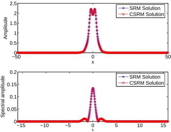
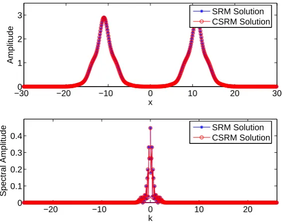
For the last assessment, we compare the N = 512 component SRM and the M =

(11)

−300 −20 −10 0 10 20 30 1

2 3

x

Amplitude

−20 −10 0 10 20

0 0.1 0.2 0.3 0.4

k

Spectral Amplitude

Figure 8. Comparison of N = 512 component SRM and M = 64 component CSRM solutions for a) dual soliton b) their spectra

two Gaussian with unit amplitudes located at −10 and 10. As before, the upper bound

for the convergence criteria ofα is selected as 10−5. Both the SRM and CSRM converges

to the depicted solution after few iteration steps. For this case, the normalized

root-mean-square difference using the SRM and the CSRM solutions is 4.80×10−3in physical domain

and 1.40×10−3 in the Fourier domain. The two methods are in acceptable agreement

as it can be seen in the figure. Compared to the previous cases, the increase in the error is due to the less number of zeros in the wider dual soliton profile compared to single soliton, which causes the sparsity condition of the CS to be violated. The potential term has also an effect on the violation of CS since it affects the soltion shapes. It is natural to expect that with higher undersampling ratios (i.e. more missing spectral data), the error will increase and CSRM may eventually fail as discussed before for the case depicted in Figure 4. However the capability of CSRM to capture self-localized solutions despite these large undersampling ratios shows that CSRM can be a very useful method in evaluating self-localized solutions in many systems with missing spectral data. This method can also be generalized to many other nonlinear system of equations used to describe many different physical phenomena and can also be applied to other periodic or nonperiodic domain spectral methods for evaluating computational solutions under missing spectral or pseudospectral data.

4. Conclusion and Future Work

In this paper we have proposed a novel numerical scheme for finding the sparse self-localized states of a nonlinear system of equations when there is missing spectral data. The

method utilizes far fewer number of spectral components (M) than classical versions of the

Petviashivili’s method or spectral renormalization method with higher number of spectral

components (N). After the converge criteria is achieved for M components, the signal

with N components can be reconstructed from M components by the l1 minimization

(12)

spectral renormalization (CSRM) method. Compared to SRM, the main advantage of the CSRM is that, it is capable of finding the sparse self-localized states of the evolution equation(s) with far fewer spectral data. For example for fiber optical communications, where some data is lost during the propagation of the optical pulse or considering memory and time constraints they may be intentionally ignored, CSRM can be used to find self localized states of the system of equations studied. CSRM can also be computationally

advantageous depending on how largeN−M is and the number of iteration steps needed

to obtain a convergent solution but for a more general extension of SRM, where soliton eigenvalue depends of propagation distance, this advantage would be more clear. For such a case application of SRM at each along fiber point would be necessary thus CSRM would also be computationally very advantageous while there would be negligible accuracy difference between CSRM and SRM.

There are some sparse FFT algorithms well developed and used in the literature. As a future work it is possible to implement these sparse fast transforms for computational modeling of the sparse signals and provide a comparison with the CSRM. The sequential, parallel or distributed algorithms can be used for this purpose. The CSRM can also be incorporated for other type of spectral methods such as those where the wavelets, DCTs, Legendre, Chebyshev and other forms of basis functions are used for computational simulations.

References

[1] Schoellhamer, D. H., (2001), Geophysical Research Letters,28, 16, 3187. [2] Stoica P., Li J., Ling J., (2009), IEEE Signal Processing Letters,16, 241.

[3] Thiele H. J., Nebeling M., (2007), Coarse Wavelength Division Multiplexing, CRC Press. [4] Walker S., (1986), Journal of Ligthwave Technology,4, 8, 1125.

[5] Comerford L., Kougioumtzoglou I. A., Beer M., (2016), Probabilistic Engineering Mechanics,44, 66. [6] Ablowitz M. J., Musslimani Z. H., (2005), Optics Letters, 30, 16, 2140.

[7] Zakharov V. E., (1968), Soviet Physics JETP, 2, 190.

[8] Zakharov V. E., Shabat A. B., (1972), Soviet Physics JETP,34, 62. [9] Bayındır C., (2009), MS Thesis, University of Delaware.

[10] Canuto C, (2006), Spectral Methods: Fundamentals in Single Domains, Springer-Verlag.

[11] Karjadi E. A., Badiey M, Kirby J. T., (2010), The Journal of the Acoustical Society of America,127, 1787.

[12] Karjadi E. A., Badiey M, Kirby J. T., Bayındır C., (2012), IEEE Journal of Oceanic Engineering,

37-1, 112.

[13] Trefethen L. N., (2000), Spectral Methods in MATLAB, SIAM. [14] Bayındır C., (2016), Physical Review E.,93, 032201.

[15] Bayındır C., (2016), Physical Review E,93, 062215. [16] Bayındır C., (2016), Physics Letters A,380, 156.

[17] Bayındır C., (2016), TWMS Journal of Applied and Engineering Mathematics,6-1, 135. [18] Demiray H., Bayındır C., (2015), Physics of Plasmas,22, 092105.

[19] Bayındır C., (2016), arXiv Preprint, arXiv: 1604.06604. [20] Bayındır C., (2016), arXiv Preprint, arXiv: 1602.05339. [21] Bayındır C., (2016), arXiv Preprint, arXiv: 1602.00816. [22] Bayındır C., (2016), arXiv Preprint, arXiv: 1512.03584.

[23] Petviashvili V. I., (1976), Soviet Journal of Plasma Physics JETP,2, 257. [24] T. I. Lakoba, Yang J., (2007), Journal of Computational Physics,226, 1668.

[25] Fibich G., (2015), The Nonlinear Schrodinger Equation: Singular Solutions and Optical Collapse, Springer-Verlag.

[26] Antar N., (2014), Journal of Applied Mathematics,848153.

[27] Goksel I., Antar N., Bakirtas I., (2018), Chaos, Solitons & Fractals,109, 83.

(13)

[31] Bayındır C., (2016) Sci. Rep.,6, 22100; doi: 10.1038/srep22100.

[32] Bayındır C., (2015), TWMS Journal of Applied and Engineering Mathematics,5-2, 298.

[33] Bayındır C., (2015), Hesaplamalı Akı¸skanlar Mekani˘gi Ç alı¸smaları i¸cin Sıkı¸stırılabilir Fourier Tayfı Yöntemi, XIX. Türk Mekanik Kongresi, Trabzon. (In Turkish)

[34] Bayındır C., (2015), Okyanus Dalgalarının Sıkı¸stırılabilir Fourier Tayfı Y¨ontemiyle Hızlı Modellenmesi, XIX. T¨urk Mekanik Kongresi, Trabzon. (In Turkish)

Cihan Bayındırfor the photography and short autobiography, see TWMS J. App. Eng. Math., V.5,