FUNCTION AND DIVERSITY ACROSS SPATIAL SCALES FROM FULL WAVEFORM LIDAR
by
Ginikanda Yapa Mudiyanselage Nayani Thanuja Ilangakoon
A dissertation
submitted in partial fulfillment of the requirements for the degree of Doctor of Philosophy in Geosciences
Boise State University
© 2020
Ginikanda Yapa Mudiyanselage Nayani Thanuja Ilangakoon ALL RIGHTS RESERVED
DEFENSE COMMITTEE AND FINAL READING APPROVALS
of the dissertation submitted by
Ginikanda Yapa Mudiyanselage Nayani Thanuja Ilangakoon
Dissertation Title: Complexity and Dynamics of Semi-arid Vegetation Structure, Function and Diversity Across Spatial Scales from Full Waveform Lidar
Date of Final Oral Examination: 20 February 2020
The following individuals read and discussed the dissertation submitted by student Ginikanda Yapa Mudiyanselage Nayani Thanuja Ilangakoon, and they evaluated her presentation and response to questions during the final oral examination. They found that the student passed the final oral examination.
Nancy F. Glenn, Ph.D. Chair, Supervisory Committee
Shawn Benner, Ph.D. Member, Supervisory Committee
Jodi Brandt, Ph.D. Member, Supervisory Committee
Dylan Mikesell, Ph.D. Member, Supervisory Committee
The final reading approval of the dissertation was granted by Nancy F. Glenn, Ph.D., Chair of the Supervisory Committee. The dissertation was approved by the Graduate College.
iv
This dissertation is dedicated to my wonderful daughter Amelia and to
my Appachchi (Dad), the strength of my life.
v
I would like to express my deepest appreciation and gratitude to my advisor Dr. Nancy F. Glenn for her guidance, support, and patience throughout this journey. I would also like to convey sincere thanks to the dissertation committee: Dr. Shawn Benner, Dr. Jodi Brandt, and Dr. Dylan Mikesell for their enormous support and constructive feedback during my PhD.
I would like to thank the NASA Terrestrial Ecology (NASA TE -NNX14AD81G) and the NASA Earth and Space Science Fellowship (NESSF - 17-EARTH17F-0209) programs for supporting me with funding.
I sincerely appreciate Dr. Thomas Painter, Dr. Cathie Olschanowsky, Dr. Fabian Schneider, Dr. Steven Hancock, and Dr. Tristan Goulden, for their invaluable support during my PhD including journal publications.
Thank you to USDA ARS Northwest Watershed Research Center for access and support to Reynolds Creek Experimental Watershed (RCEW) where this study took place.
I would like to thank all BCAL group members for their generous support during my PhD.
I would also like to thank Boise State Research Computing for their enormous support and co-operation with me when I use many cores of the cluster at the same time. I convey my gratitude to the faculty, staff, and students of the Department of Geosciences for their help during my stay at Boise State University.
vi by me during this journey.
vii
Semi-arid ecosystems cover approximately 40% of the earth’s terrestrial landscape and show high dynamicity in ecosystem structure and function. These ecosystems play a critical role in global carbon dynamics, productivity, and habitat quality. Semi-arid ecosystems experience a high degree of disturbance that can severely alter ecosystem services and processes. Understanding the structure-function
relationships across spatial extents are critical in order to assess their demography, response to disturbance, and for conservation management. In this research, using state-of-the-art full waveform lidar (airborne and spaceborne) and field observations, I developed a framework to assess the complexity and dynamics of vegetation structure, function and diversity across spatial scales in a semi-arid ecosystem.
Difficulty in differentiating low stature vegetation from bare ground is the key remote sensing challenge in semi-arid ecosystems. In this study, I developed a workflow to differentiate key plant functional types (PFTs) using both structural and biophysical variables derived from the full waveform lidar and an ensemble random forest technique. The results revealed that waveform lidar pulse width can clearly distinguish shrubs from bare ground. The models showed PFT classification accuracy of 0.81–0.86% and 0.60– 0.70% at 10 m and 1 m spatial resolutions, respectively. I found that structural variables were more important than the biophysical variables to differentiate the PFTs in this study area. The study further revealed an overlap between the structural features of different PFTs (e.g. shrubs from trees).
viii
plant area index and foliage height diversity) of shrubs and trees that describe canopy architecture and light use efficiency of the ecosystem. I evaluated the trends and patterns of functional diversity and their relationship with non-climatic abiotic factors and fire disturbance. In addition to the fine resolution airborne lidar, I used simulated large footprint spaceborne lidar representing the newly launched Global Ecosystem Dynamics Investigation system (GEDI, a lidar sensor on the International Space Station) to evaluate the potential of capturing functional diversity trends of semi-arid ecosystems at global scales. The consistency of diversity trends between the airborne lidar and GEDI confirmed GEDI’s potential to capture functional diversity. I found that the functional diversity in this ecosystem is mainly governed by the local elevation gradient, soil type, and slope. All three functional diversity indices (functional richness, functional evenness and functional divergence) showed a diversity breakpoint near elevations of 1500 m – 1700 m. Functional diversity of fire-disturbed areas revealed that the fires in our study area resulted in a more even and less divergent ecosystem state. Finally, I quantified aboveground biomass using the structural features derived from both the airborne lidar and GEDI data. Regional estimates of biomass can indicate whether an ecosystem is a net carbon sink or source as well as the ecosystem’s health (e.g. biodiversity). Further, the potential of large footprint lidar data to estimate biomass in semi-arid ecosystems are not yet fully explored due to the inherent overlapping vegetation responses in the ground signals that can be affected by the ground slope. With a correction to the slope effect, I found that large footprint lidar can explain 42% of variance of biomass with a RMSE of 351 kg/ha (16% RMSE). The model estimated 82% of the study area with less than 50%
ix
richness showed the highest uncertainties. Overall, this dissertation establishes a novel framework to assess the complexity and dynamics of vegetation structure and function of a semi-arid ecosystem from space. This work enhances our understanding of the present state of an ecosystem and provides a foundation for using full waveform lidar to
understand the impact of these changes to ecosystem productivity, biodiversity and habitat quality in the coming decades. The methods and algorithms in this dissertation can be directly applied to similar ecosystems with relevant corrections for the appropriate sensor. In addition, this study provides insights to related NASA missions such as
ICESat-2 and future NASA missions such as NISAR for deriving vegetation structure and dynamics related to disturbance.
x
DEDICATION ... iv
ACKNOWLEDGEMENTS ...v
ABSTRACT ... vii
TABLE OF CONTENTS ...x
LIST OF TABLES ... xiv
LIST OF FIGURES ...xv
LIST OF ABBREVIATIONS ...xx
CHAPTER ONE: INTRODUCTION ...1
CHAPTER TWO: CONSTRAINING PLANT FUNCTIONAL TYPES IN A SEMI-ARID ECOSYSTEM WITH WAVEFORM LIDAR ...7
Abstract ...7
Introduction ...8
Materials ...14
Study area...14
Field data ...15
Small-footprint waveform lidar data ...16
Methods...17
Decomposition of waveform lidar signals ...17
Additional waveform features derived from Gaussian decomposition ...19
xi
Implementation of random forest classification ...26
Results ...30
Influence of the viewing geometry on waveform features ...30
Important waveform features for PFT classification ...30
RF model performance ...34
Discussion ...35
Differentiating PFTs with waveform features ...35
Waveform derived heights and differentiating bare ground from vegetation ...41
Scale dependency of PFT classification ...42
Upscaling to large-footprint waveforms ...43
Conclusions ...45
CHAPTER THREE: SPACEBORNE LIDAR REVEALS TRENDS AND PATTERNS OF FUNCTIONAL DIVERSITY IN A SEMI-ARID ECOSYSTEM ...46
Abstract ...46
Introduction ...47
Materials and Methods ...50
Study area...50
Field data ...51
Environmental data ...52
Airborne lidar data ...52
Derivation of bare ground ...53
xii
Functional diversity ...58
Statistical analysis ...59
Results ...60
Discussion ...76
Mapping functional traits ...76
Functional diversity in semi-arid ecosystems ...78
Conclusion ...82
CHAPTER FOUR: ESTIMATING ABOVEGROUND BIOMASS IN A SEMI-ARID ECOSYSTEM FROM LARGE FOOTPRINT LIDAR DATA: INSIGHTS FOR GEDI .83 Abstract ...83
Introduction ...84
Methods...88
Study area...88
Field data ...89
Airborne lidar data (ASO) ...90
GEDI simulation ...90
Reference biomass ...92
GEDI biomass model development ...93
Results ...96
Discussion ...103
Conclusion ...109
CHAPTER FIVE: CONCLUSION...110
xiii
Supplementary figures for chapter 3 ...137 Supplementary figures for chapter 4 ...142
xiv
LIST OF TABLES
Table 2.1 Summary of waveform features derived from individual waveforms and their biophysical relationships to the target. ... 11 Table 2.2 Features extracted from waveform backscatter lidar. ... 25 Table 2.3 Ensemble random forest (E-RF) models used to evaluate the waveform
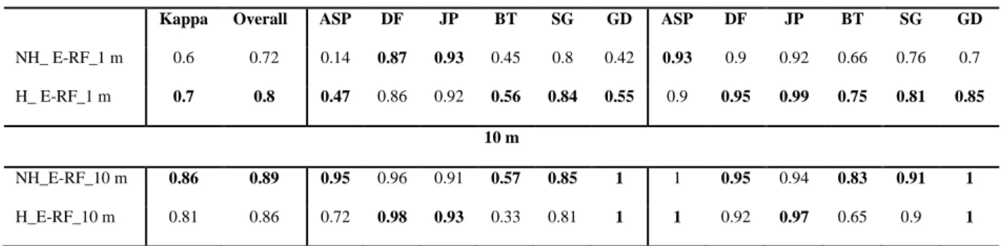
attribute selection and PFT classification. ... 29 Table 2.4 Producer and user accuracy of each PFT (ASP, DF, JP, BT, SG, and GD) in each RF model described in Table 3. ... 35
xv
LIST OF FIGURES
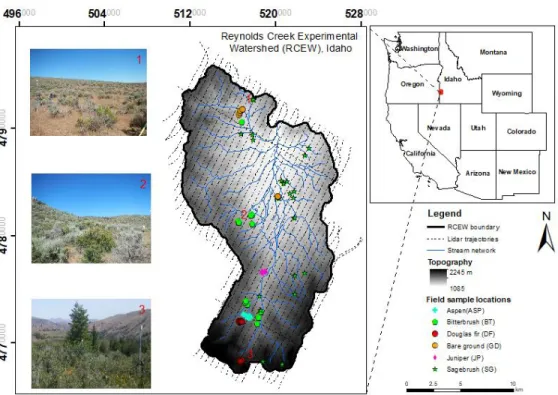
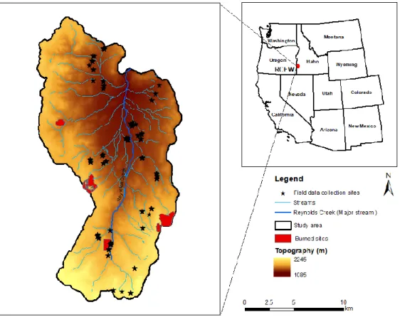
Figure 2.1 Reynolds Creek Experimental Watershed study area with field sample locations (n=103 plots) of plant functional types (ASP, DF, JP, BT, SG, and GD) and waveform lidar trajectories. Field photos depict the sparse to dense shrub and tree communities (from top to bottom photo). ... 15 Figure 2.2 Workflow illustrating the steps used to derive waveform features from the
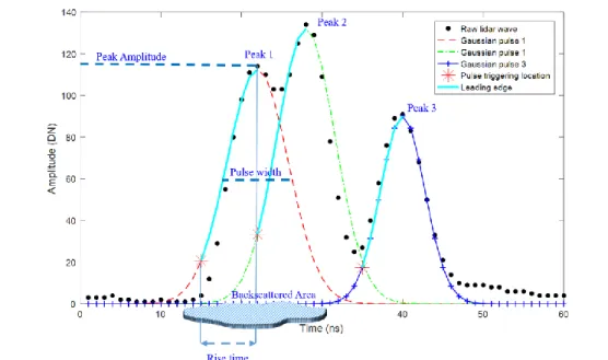
raw backscattered lidar waveform. Processing includes georeferencing, data alignment, Gaussian decomposition, deconvolution, and calibration. ... 18 Figure 2.3 Illustration of information contained in a lidar waveform. Peak 1, 2, and 3
are the echoes from three scatterers detected by the waveform. Three Gaussian functions (Gaussian pulse 1, 2, and 3) were fitted to the raw waveform. The peak amplitude is the maximum amplitude of the first echo after Gaussian fitting. Pulse width is the full width at half maximum. The stars are the trigger locations of each echo. Leading edge is the time distance from trigger to the max amplitude. The backscattered area
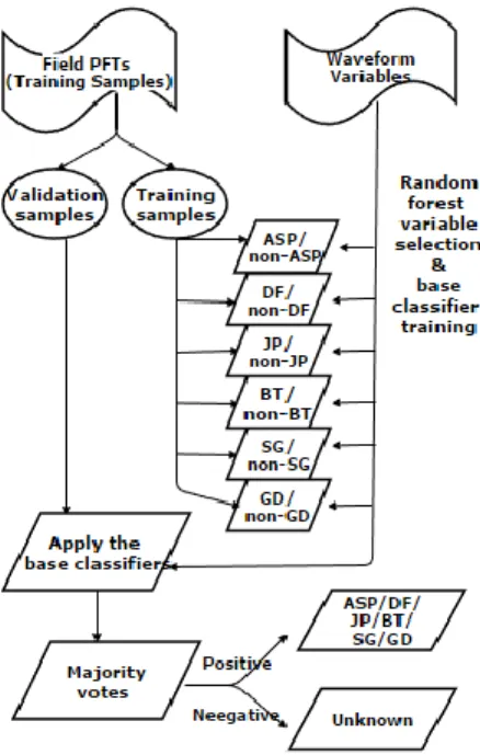
represents the scattered cross-section from the first echo. ... 24 Figure 2.4 Ensemble random forest PFT classification workflow. Feature selection
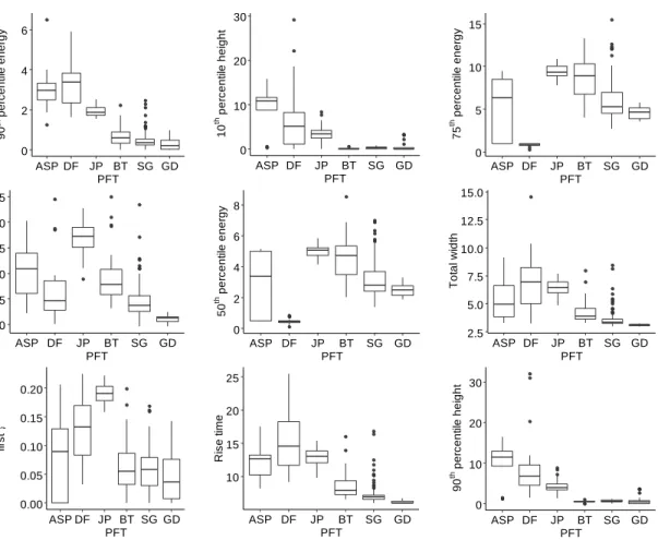
and base classifiers were trained using training samples. The selected base classifier models were applied to the validation samples and ensembled to make the final decision. ... 28 Figure 2.5 Box plots showing the variability of values of the most important
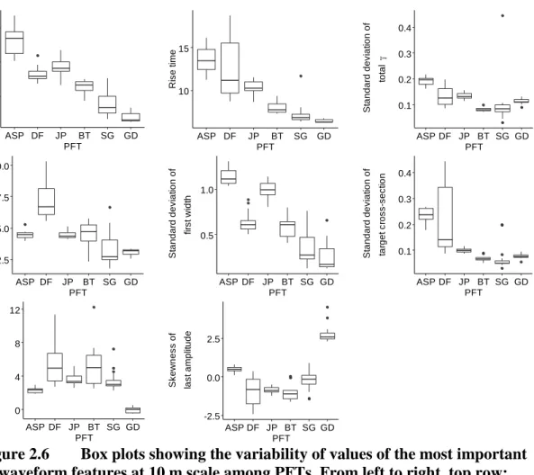
waveform features at 1 m scale among PFTs. Definitions of PFTs are: ASP-aspen, DF-Douglas fir, JP-juniper, BT-bitterbrush, SG-sagebrush, GD-bare ground. From left to right, top row: variability of standard deviation of 90th percentile energy, 10th percentile height, and 75th percentile energy, respectively; middle row: variability of pulse width of first returns (first width), 50th percentile energy, and pulse widths of all returns (total width), respectively; bottom row: variability of standard deviation of backscatter coefficient of first returns (first γ), rise time, and 90th percentile energy, respectively. Note the differentiation of shrubs and bare ground with the pulse width and rise time. ... 32 Figure 2.6 Box plots showing the variability of values of the most important
waveform features at 10 m scale among PFTs. From left to right, top row: variability of pulse width of first return, rise time, and standard deviation
xvi
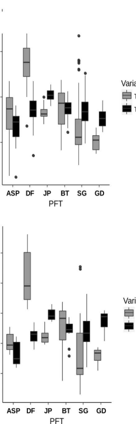
of total backscattering coefficients, respectively; middle row: variability of energy at 50th percentile height, and standard deviation of first return pulse widths, and standard deviation of target cross-section, respectively; bottom row: variability of kurtosis of first return amplitudes and skewness of last return amplitudes, respectively. ... 34 Figure 2.7 Distribution of total backscattered coefficient (total γ) and target
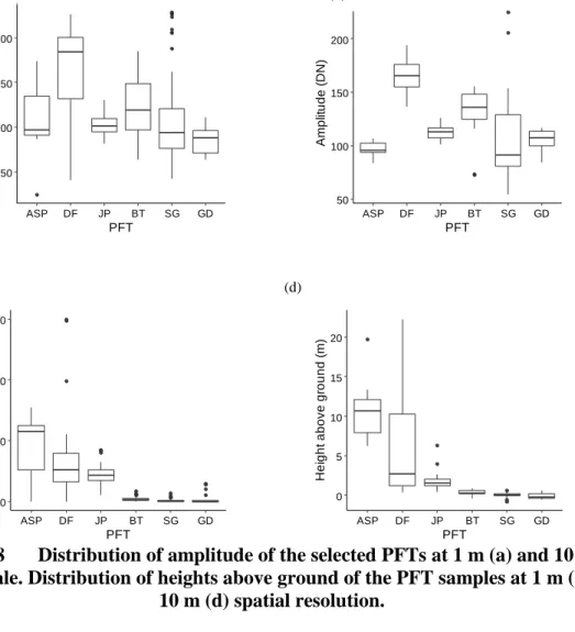
cross-section (σ) of PFTs at 1 m (a) and 10 m (b) spatial resolution. Total backscatter coefficient shows less variability than the target cross section within PFTs as well as among PFTs. ... 38 Figure 2.8 Distribution of amplitude of the selected PFTs at 1 m (a) and 10 m (b)
spatial scale. Distribution of heights above ground of the PFT samples at 1 m (c) and 10 m (d) spatial resolution. ... 40 Figure 3.1 Reynolds Creek Experimental Watershed, SW Idaho with the topographic gradient and stream network. The black stars represent 10 m x 10 m field plots across the watershed. ... 51 Figure 3.2 Summary workflow for deriving plant area index from small footprint
waveform lidar. ... 54 Figure 3.3 Correlation between a) field measured max vegetation heights and ASO
derived vegetation heights, b) field measured plant area index (PAI) and ASO derived PAI, c) field measured max vegetation heights and GEDI derived vegetation heights, and d). field measured PAI and GEDI derived PAI . ... 61 Figure 3.4 Correlation between a) field measured max vegetation heights and ASO
derived PAI, b) ASO derived FHD and ASO derived PAI, c) field measured max vegetation heights and GEDI derived PAI, and d). GEDI derived FHD and GEDI derived PAI . ... 62 Figure 3.5 ASO and GEDI derived functional traits distribution across the RCEW.
Top row: a). ASO derived PAI, b). ASO derived FHD, c). ASO derived CH. Bottom row: d). GEDI derived PAI, e). GEDI derived FHD, f). GEDI derived CH. The ASO based maps were derived at 10 m spatial resolution. GEDI data are displayed at footprint scale. The ASO and GEDI canopy heights are displayed as log canopy heights to enhance the visualization of canopy height distribution across the study area. ... 65 Figure. 3.6 Functional diversity derived using 500 m spatial neighborhood from ASO
(top row- richness, evenness, divergence), and GEDI (bottom row- richness, evenness, divergence). Functional richness, functional evenness and functional divergence of RCEW derived from functional traits
xvii
distribution across 500 m neighborhood to each 10 m x 10 m pixel in ASO and 25 m x 25 m footprints in GEDI. ... 66 Figure. 3.7 Correlation between ASO and GEDI based diversity indices at 500 m
spatial neighborhood. ... 67 Figure. 3.8 Functional diversity – environmental gradient trends of RCEW. The red
and blue curves represent the mean variation of diversity indices from ASO and GEDI respectively and the surrounding gray area represents the standard deviation. From top to bottom variation of functional diversity with altitude (a,b,c), aspect (d,e,f), slope (g,h,i), topographic wetness index (TWI) (j,k,l), and distnace to water (m,n,o) are displayed. ... 70 Figure. 3.9Variance of functional diversity explained by each abiotic factor; a). ASO
functional richness, b). ASO functional evenness, c). ASO functional divergence, d). GEDI functional richness, e). GEDI functional evenness, f). GEDI functional divergence. TWI – topographic wetness index, DTW – distance to the nearest stream in meters. ... 70 Figure. 3.10 Frequency distribution of functional traits within the fire disturbed and
surrounding undisturbed areas of RCEW. The pink represents the functional traits from burned areas while the green represents the
functional traits of undisturbed areas. ... 72 Figure. 3.10 Frequency distribution of functional diversity indices of burned and
unburned areas of RCEW. The pink represents the functional diversity from burned areas while the green represents the functional diversity of undisturbed areas. ... 73 Figure. 3.11 Functional diversity variability with search neighborhood radius at four
different burned regions. Pink represents the burned areas and the blue represents the surrounding unburned areas. ... 75 Figure. 4.1 Assimilation of vegetation signal with ground signal in large footprint
lidar data over sloped terrain. ... 87 Figure. 4.2 a) Reynolds Creek Experimental Watershed (RCEW) study area
vegetation. b) ASO derived reference biomass distribution. The red dots in a) represents the spatial distribution of field plots. ... 89 Figure. 4.3 Processing workflow of GEDI biomass and biomass uncertainty estimates. ... 95 Figure. 4.4 ASO point cloud derived a) maximum vegetation heights and, b) percent
xviii
Figure. 4.5 Correlation coefficients between slope corrected GEDI RH metrics and field observed max vegetation heights. ... 97 Figure. 4.6 Reference ASO biomass versus predicted GEDI footprint biomass (kg/ha) with the 1:1 line. ... 99 Figure. 4.7 a) ASO reference biomass with vegetation above 3m masked and b)
predicted GEDI footprint biomass. ... 100 Figure. 4.8 a) GEDI footprint level biomass; and b) prediction uncertainty from the
95% credible interval; and c) percent uncertainty. ... 101 Figure. 4.9 ASO and GEDI biomass comparison including a) reference ASO biomass resampled to 1 km; b) predicted GEDI biomass resampled to 1 km; and c) biomass differences between reference and GEDI at 1 km. ... 102 Figure. 4.10 Uncertainty of biomass with upscaling to 1 km including a) predicted
GEDI footprint level biomass; b) range of biomass within each 1 km pixel and c) standard deviation of biomass at 1 km pixels derived from the 25 m footprint biomass. ... 103 Figure. 4.11 A sample simulated GEDI waveform with the reference ASO waveform
and the cumulative energy profile. The reference ASO waveform is contained within the GEDI RH16 and RH68. ... 104 Figure. 4.12 Correlation of percent uncertainty with mean footprint vegetation height
and percent vegetation cover. ... 107 Figure. 4.13 GEDI footprint density and standard deviation of biomass at 1 km pixels.
... 108 Figure S.1 Boxplots of CH, PAI, and FHD derived from GEDI of burned and
surrounding unburned areas of Koke fire (a, b, c), Whiskey fire (d, e, f), Break fire (g, h, i), and Rabbit Creek fire (j, k, l). ... 138 Figure S.2 Boxplots of functional richness, functional evenness, and functional
divergence calculated using GEDI functional traits of burned and surrounding unburned areas of Koke fire (a, b, c), Whiskey fire (d, e, f), Break fire (g, h, i), and Rabbit Creek fire (j, k, l). The first column represents functional richness while the second and third columns
represent functional evenness and functional divergence respectively. . 139 Figure S.3 GEDI footprints colored by functional diversity of the four different fires
studied. The first column represents functional richness while the second and third columns represent functional evenness and functional divergence respectively. ... 140
xix
Figure S.4 RCEW precipitation and temperature variation with elevation gradient. Precipitation: average for the period of 1963-2010, temperature: mean normal air temperature for the period of 1984 – 2014 (PRISM Climate Group, 2016, CZO Dataset: Reynolds Creek, 2016) ... 141 Figure S.5 Frequency distribution of a) predicted GEDI biomass and b) percent
uncertainty at GEDI footprint scale. ... 142 Figure S.6 Variance of predicted footprint biomass and percent uncertainty explained by Slope, Vegetation heights and percent vegetation cover. ... 142
xx
LIST OF ABBREVIATIONS
ASO Airborne Snow Observatory
AGB Aboveground biomass
ALS Airborne laser scanning
ASP Aspen
BT Bitterbrush
CH Canopy height
CHM Canopy height models
DEM Digital elevation models
DTW Distance to water
FHD Foliar height diversity
GD Bare ground
GEDI Global Ecosystem Dynamic Investigation
DF Douglas fir
JP Juniper
PAI Plant Area Index
PFT Plant functional types
NASA National Aeronautics and Space Administration
SG Sagebrush
CHAPTER ONE: INTRODUCTION
Over the last few decades, land degradation has become a critical challenge for terrestrial ecosystems. Climate and human driven disturbances modify the structure and function of natural ecosystems. Altered ecosystem structure and function provide adverse effects on ecosystem services and processes including productivity, biodiversity and habitat quality. Understanding the structure and function of global terrestrial ecosystems improves the understanding of their interactions with the biosphere, atmosphere, and hydrosphere including the cycling of the major biogeochemical elements and water (Diaz et al., 2007; Dietze et al., 2017). Further, assessing the effects of climate and human driven changes at different levels provide necessary information for national and
international policy discussion around mitigation targets (Arnell, Lowe, Challinor, &
Osborn, 2019; Rödig et al., 2019). Quantitative assessments of ecosystem structure, function and their spatial diversity at regional to global scales are fundamental to monitor the ecosystem state, and the impact to the atmosphere, biosphere, and hydrosphere under changing conditions. Among others, semi-arid ecosystems experience a high degree of land degradation (Fusco, Rau, Falkowski, Filippelli, & Bradley, 2019) due to both climatic (drought, fire, invasion and encroachment, erosion etc.) and anthropogenic (grazing, land use, agriculture) disturbances. Semi-arid ecosystems cover approximately 40% of the global terrestrial surface and are home to about 20% of the world’s population (Li et al., 2018; (Nautiyal, Bhaskar, & Khan, 2015). These ecosystems are typically heterogeneous, low-stature, and sparsely vegetated. Semi-arid ecosystems comprise a
range of intra and inter species structural and functional characteristics. These
heterogeneous vegetation characteristics provide habitat and biodiversity to unique fauna and flora as well as two billion people worldwide (Nautiyal, Bhaskar, & Khan, 2015). Further, semi-arid ecosystems play a critical role in global carbon dynamics (Ahlstrom et al., 2015; Poulter et al., 2015) and show that afforestation could offset the climate
warming effects and cool the planet (Yosef et al., 2018).
Availability of remote sensing data at fine to coarse spatial and temporal scales facilitates monitoring the retrospective and prospective states of ecosystems across spatial scales needed for ecosystem service management (Abelleira Martínez et al., 2016). Importantly, waveform lidar, which digitizes the total amount of lidar return energy at high vertical resolution (~1 ns = 15 cm) provides unprecedented opportunities to accurately quantify ecosystem structure and function at local to regional scales ( Hovi, Korhonen, Vauhkonen, & Korpela, 2016; Qi, Lee, et al., 2019; Yao, Krzystek, & Heurich, 2012). With the launch of the Global Ecosystem Dynamics Investigation (GEDI) mission, we have new opportunities to map functional types, traits and diversity at global scales (Duncanson et al., 2019; Qi, Lee, et al., 2019; Qi et al., 2019; Rödig et al., 2019).
The abundance and distribution of plant functional types (PFTs) are important indicators for monitoring ecosystem state, as well as its resistance and resilience to climate and human driven disturbances (Lavorel, McIntyre, Landsberg, & Forbes, 1997; Poulter et al., 2015; Schimel, Asner, & Moorcroft, 2013). Thus, PFTs are frequently used as inputs for vegetation dynamics and earth system models (Krinner et al., 2005; Sitch et al., 2003; Wullschleger et al., 2014). However, uncertainty in PFTs, especially in
semi-arid ecosystems between shrub, grass and forest classes reduces the accuracy of these models (Hartley, MacBean, Georgievski, & Bontemps, 2017). In semi-arid ecosystems, the influence of soil background on the remote-sensing signals is a major challenge. Improved methods to capture plant functional types (PFTs) in semi-arid ecosystems are needed to accurately assess the ecosystem state.
A wealth of research has shown that functional traits are the best representatives of ecosystem processes (Bardgett & van der Putten, 2014; Hooper et al., 2006). Research evidence further indicates that, though net primary productivity (NPP), nutrient retention, and disturbance regimes can describe facets of ecosystem functioning, none of these variables can directly quantify the observed diversity in ecosystem functioning (Gough et al., 2016). Moreover, disturbance-driven alterations and their ecological impacts are highly dynamic in space and time. Morphological, physiological and phenological traits within and between species of an ecosystem can represent the ecosystem demography and response strategies to the disturbances (Serbin et al., 2019). Thus, remotely sensed functional traits and their diversity are widely utilized in forested ecosystems to predict variations in ecosystem structure – function relationships (Funk et al., 2017, Wieczynski et al., 2019). Yet, several gaps remain in our understanding of how the complexity and dynamics of functional diversity in semi-arid ecosystems vary with respect to the environmental gradient and in response to disturbance, especially post fire.
Another important vegetation functional trait is the canopy aboveground biomass (ABG). AGB serves to characterize, quantify, understand, and predict whether
ecosystems are a net carbon sink or source (Duncanson et al., 2019; Li et al., 2015; Qi et al., 2019). Hence, accurate estimates of ABG at regional to global scales improves the
understanding of carbon fluxes associated with the ecosystem and provides significant implications to constrain global vegetation/carbon dynamics. AGB can further help assess ecosystem health including biodiversity. Fusco, Rau, Falkowski, Filippelli, & Bradley, (2019) demonstrated that both shrublands and woodlands account for significant carbon storage, especially in semi-arid ecosystems. Ahlström et al. (2015) showed that semi-arid ecosystems control inter-annual variability of global carbon. Nevertheless, estimating ABG from remote sensing data, especially over semi-arid ecosystems at regional scale has been a long-standing challenge due to the short canopies and their sparse distribution in space.
The overarching goal of this dissertation is to develop novel remote sensing-based methods for and to understand the complexity and dynamics of the vegetation structure, function and diversity across spatial scales in a semi-arid ecosystem. To address this, three main research questions are considered, including:
1. How can key plant functional types including shrubs, trees, and bare ground be differentiated using state-of-the-art full waveform lidar data?
2. What are the trends and patterns of functional diversity in the study area and their abiotic controls?
a. What is the potential of the newly launched GEDI, the spaceborne lidar system to capture functional diversity trends in a semi-arid ecosystem?
3. What is the uncertainty of regional AGB estimates in semi-arid ecosystems using the GEDI system?
For a test study area, I used the Reynolds Creek Experimental Watershed (RCEW), a semi-arid ecosystem of approximately 270 km2 within the Great Basin ecoregion in the Western US. The RCEW has a range of topography (1100 m – 2200 m) and a diverse vegetation community. While the unique and important sagebrush-steppe with many grass and forbs dominates the low elevations, tree communities mark the high elevations. In addition, riparian vegetation with cottonwood and willow are found within valleys, and along streams across the watershed. The study area is further characterized by a mean annual temperature and precipitation that varies between 4.6–9.2 ⁰ C and 230-959 mm, along the elevation gradient, respectively. The study area has experienced prescribed and natural fires and supports grazing. Consequently, invasion of cheatgrass in native shrub areas and juniper encroachment have occurred in this study area during the last few decades. The diverse topography, vegetation, and disturbance followed by invasion history of the study area provided a unique setting to elucidate the main research questions of this dissertation.
To answer the research questions, I first developed a novel methodological workflow for state-of-the-art full waveform lidar to differentiate key plant functional types. In this, I decoded structural and biophysical characteristics of vegetation and bare ground embedded in the lidar signal (Chapter 2). Then, I investigated the relationships between both functional diversity and environmental gradients (altitude, slope, aspect, topographic wetness index, and distance to water) and functional diversity and disturbance
relationships (e.g. fire). This work focuses on understanding the ecosystem demography and response strategies to disturbance (Chapter 3). Finally, I estimated the uncertainty in assessing the AGB of this heterogeneous, low-stature, semi-arid ecosystem (Chapter 4).
In this, I used spatially explicit vegetation structure derived from simulated GEDI lidar, especially in support of new measurement capabilities for satellite missions and global vegetation/carbon dynamics.
CHAPTER TWO: CONSTRAINING PLANT FUNCTIONAL TYPES IN A SEMI-ARID ECOSYSTEM WITH WAVEFORM LIDAR
This chapter has been published as:
Ilangakoon, N. T., Glenn, N. F., Dashti, H., Painter, T. H., Mikesell, T. D., Spaete, L. P., Jessica J. Mitchell, & Shannon, K. (2018). Constraining plant functional types in a
semi-arid ecosystem with waveform lidar. Remote Sensing of Environment, 209, 497-509.
Abstract
Accurate classification of plant functional types (PFTs) reduces the uncertainty in global biomass and carbon estimates. Airborne small-footprint waveform lidar data are increasingly used for vegetation classification and above-ground carbon estimates at a range of spatial scales in woody or homogeneous grass and savanna ecosystems. However, a gap remains in understanding how waveform features represent and
ultimately can be used to constrain the PFTs in heterogeneous semi-arid ecosystems. This study evaluates lidar waveform features and classification performance of six major PFTs, including shrubs and trees, along with bare ground in the Reynolds Creek Experimental Watershed, Idaho, USA. Waveform lidar data were obtained with the NASA Airborne Snow Observatory (ASO). From these data we derived waveform features at two spatial scales (1 m and 10 m rasters) by applying a Gaussian
decomposition and a frequency-domain deconvolution. An ensemble random forest algorithm was used to assess classification performance and to select the most important
waveform features. Classification models developed with the 10 m waveform features outperformed those at 1 m (Kappa (κ) = 0.81–0.86 vs. 0.60–0.70, respectively). At 1 m resolution, lidar height features improved the PFT classification accuracy by 10% compared to the analysis without these features. However, at 10 m resolution, the inclusion of lidar derived heights with other waveform features decreased the PFT classification performance by 4%. Pulse width, rise time, percent energy, differential target cross section, and radiometrically calibrated backscatter coefficient were the most important waveform features at both spatial scales. A significant finding is that bare ground was clearly differentiated from shrubs using pulse width. Though the overall accuracy ranges between 0.72 – 0.89 across spatial scales, the two shrub PFTs showed 0.45 - 0.87 individual classification success at 1 m, while bare ground and tree PFTs showed high (0.72 – 1.0) classification accuracy at 10 m. We conclude that small-footprint waveform features can be used to characterize the heterogeneous vegetation in this and similar semi-arid ecosystems at high spatial resolution. Furthermore, waveform features such as pulse width can be used to constrain the uncertainty of terrain modeling in environments where vegetation and bare ground lidar returns are close in time and space. The dependency on spatial resolution plays a critical role in classification performance in tree-shrub co-dominant ecosystems.
Introduction
Climate and human driven disturbances in dryland ecosystems have adverse effects on biodiversity, ecosystem services, carbon storage, and desertification (Ahlstrom et al., 2015; Poulter et al., 2011). Furthermore, aridity in drylands is expected to increase in the future, causing expansion of land degradation and desertification (Huang et al.,
2017). Ultimately, changes in the abundance and distribution of plant functional types (PFTs) in drylands can alter productivity and the capacity of these lands for carbon storage (Chen et al., 2017). Thus, PFTs are important indicators for monitoring the state of an ecosystem, as well as its resistance and resilience to climate and human driven disturbances (Lavorel et al., 1997; Poulter et al., 2015; Schimel, Asner, & Moorcroft, 2013). PFTs are frequently used as inputs for vegetation dynamics and earth system models (Krinner et al., 2005; Sitch et al., 2003; Wullschleger et al., 2014). However, uncertainty in PFTs, especially in dryland ecosystems between shrub, grass and forest classes reduces the accuracy of these models (Hartley et al., 2017). Hence, improved methods to capture the structure and function of PFTs in drylands are needed to accurately model carbon storage flux in these systems.
Due to its ability to capture three dimensional structure and some radiometric properties, light detection and ranging (lidar) is used to derive vegetation heights and digital terrain models, as well as to classify vegetation species, function and structure (Dalponte & Coomes, 2016). These products are further used for automated forest
inventory estimates such as biomass and carbon stocks (Coomes et al., 2017; Dalponte & Coomes, 2016; Ene et al., 2017), as well as for ecosystem demography models (Thomas et al., 2008) to estimate carbon flux. Waveform lidar, which digitizes the total amount of lidar return energy at high vertical resolution (~1 ns = 15 cm), provides potential species-specific information about the illuminated target (Hancock et al., 2015; Hancock, Disney, Muller, Lewis, & Foster 2011; Roncat, Bergauer, & Pfeifer, 2011; Wagner, Ullrich, Ducic, Melzer, & Studnicka, 2006). The shape of the returning waveform results from a convolution of the temporal shape of the emitted pulse and system impulse (together
called “system response/waveform”) with the target cross-section. Thus the backscattered waveform contains target characteristics such as size, orientation, and spatial
arrangement, as well as radiometric characteristics of individual vegetation species (Hovi & Korpela, 2014; Korpela, Hovi, & Korhonen, 2013; Wagner et al., 2006).
Each echo in a waveform signal corresponds to an individual reflection target or set of targets. Thus, an echo can be used to detect individual target properties, the position and the orientation in 3D space. Through optimal waveform processing techniques, such as the commonly used Gaussian decomposition (Wagner et al., 2006), linear fitting or other asymmetric fitting techniques (Jutzi & Stilla, 2006; Mallet et al., 2010; Roncat et al., 2011; Wu, van Aardt, & Asner, 2011), numerous features can be derived from backscattered waveforms. Some of these additional waveform features and their biophysical relationships to the target are summarized in Table 2.1.
However, many of these waveform features (e.g. amplitude, pulse width, and backscatter cross section) are sensitive to system parameters such as incident angle, range and flying height (Abed, Mills, & Miller, 2012; Hovi & Korpela, 2014; Lin, 2015;
Wagner, 2010). Thus, it is necessary to correct the influence of these system parameters on waveform features prior to application (Bruggisser, Roncat, Schaepman, & Morsdorf, 2017; Fieber et al., 2013; Wagner, 2010).
Table 2.1 Summary of waveform features derived from individual waveforms and their biophysical relationships to the target.
ATTRIBUTE BIOPHYSICAL RELATIONSHIP REFERENCE
Pulse width Surface roughness and slope Fieber et al., 2013 Amplitude Optical response of the target to the emitted
lidar wavelength
Fieber et al., 2013 Backscatter
cross-section
Horizontal scattered cross-section of the target with respect to the deployed system wavelength, range, and incident angle
Wagner et al., 2006
Backscatter coefficient The area-normalized backscatter cross-section corrected for incidence angle. A function of the target reflectance.
Wagner, Hollaus, Briese, & Ducic, 2008; Wagner, 2010
Differential target cross section
Laser system independent true target profile Roncat et al., 2011 Rise time Vertical structural distribution of target (e.g.
in trees the vertical distribution of leaves and branches)
Ranson & Sun, 2000
Number of echoes Vertical distribution and height of target Heinzel & Koch, 2011
Height/height variability
Vertical distribution of target and its separation from ground
Fieber et al. 2013 Secondary explanatory
features derived from any of the above parameters
N/A Heinzel & koch,
2011
Waveform features and height information have been used to estimate vegetation structure as well as plant functional type and structural traits at both fine (< 2 m) and regional spatial scales (Alexander, Deák, Kania, Mücke, & Heilmeier, 2015; Wagner, Hollaus, Briese, & Ducic, 2008). Classification of plant functional types and individual species in tree dominant ecosystems show great improvement of classification accuracy
with inclusion of one or several of these waveform features (Hovi et al., 2016). The pulse width and location characterize the vegetation components along the waveform path and have been used to classify deciduous and coniferous species (Reitberger, Krzystek, & Stilla, 2008; Yao, Krzystek, & Heurich, 2012). Wagner et al. (2008) shows that the scattering shape of backscattered signals can be used to separate vegetation from no vegetation with an accuracy up to 89%. Pulse widths can be used to classify
vegetation in different patch conditions such as within varying soil roughness, understory and density (Hollaus, Aubrecht, Höfle, Steinnocher, & Wagner, 2011). Vaughn, Moskal, & Turnblom (2012) show that inclusion of frequency-domain full-waveform lidar
features improve a five-species classification accuracy by 6% over discrete-return lidar alone, from 79 to 85%.
Numerous studies using combined features from discrete and waveform datasets have improved classification performance of tree and grass species (Heinzel and Koch, 2011; Neuenschwander, 2009; Vaughn et al., 2012). Backscatter cross-section alone can be used to distinguish ground, grass, and trees from each other (Fieber et al., 2013; Wagner et al., 2008). Further, lidar-derived height and energy related features have been used to delineate individual trees in object-based image analysis (OBIA) studies as the OBIA eliminates the discontinuity that is common in pixel-based classification (Zahidi, Yusuf, Hamedianfar, Shafri, & Mohamed, 2015).
In most of these studies, lidar-derived heights or height-based products such as canopy height models (CHM) and digital elevation models (DEM) play a critical role in delineation of individual tree crowns as well as in differentiating vegetation from bare ground (Hovi et al., 2016). Some vegetation studies use lidar returns above a certain
height threshold (e.g. ~ 2 m above ground) for classification (Ene et al., 2017; Zahidi et al., 2015). However, in low-height vegetation, lidar does not return a separate energy peak unless the vegetation height is above the range resolution of the lidar system. Thus, bare ground lidar responses are typically mixed with low-height vegetation such as shrubs and grasses. This causes difficulties to measure the fractions of bare ground and vegetation, an important criterion for plant functional distribution mapping in dryland ecosystems (Hartley et al., 2017). Numerous studies in low-height ecosystems have documented that lidar heights underestimate vegetation heights (e.g. Streutker & Glenn, 2006). Similar underestimations and uncertainties appear in almost all studies which use lidar-based height features to model low-stature vegetated ecosystems across the world, which significantly affects regional ecosystem modeling and upscaling attempts
(Hopkinson et al., 2005; Rango et al., 2000). Fortunately, waveform lidar is sensitive to the occurrence of low vegetation, where echoes often have a wider pulse than echoes from the bare ground. Although this limits the use of traditional lidar heights to separate ground from vegetation, the derivation of additional waveform features provides the opportunity to uncover hidden vegetation characteristics in the datasets.
In addition, vegetation distributions in many semi-arid ecosystems are topographically controlled and low-height vegetation often coexist with taller tree communities. The topographic and species complexity in these ecosystems makes classification using optical data challenging. In many instances, classification studies, even at high spatial resolution, consider all shrub species in one category (e.g. Zahidi et al., 2015). The complexity of heterogeneous semi-arid ecosystems further emphasizes the importance of understanding the effects of resolution in retrieving species type and
diversity to guide future trade-offs in spaceborne sensors (e.g. GEDI and ICESat-2) (Abdalati et al., 2010; Endres, 2016; Qi & Dubayah, 2016) and ultimately, global
ecosystem modeling. Semi-arid ecosystems cover a significant portion of the global land surface, and thus, the ability to map the density of shrubs and trees in these ecosystems will advance dynamic global vegetation models that account for vegetation demography (Fisher et al. 2018). For example, the clumping of foliage affects the exposure of bare ground and ultimately the land surface water vapor, carbon, and energy exchange.
The objectives of this study are three-fold. First, we aim to identify
small-footprint waveform features to distinguish characteristics of two major shrub types from each other, from bare ground and from three dominant tree species in a pixel-based classification scheme in the Reynolds Creek Experimental Watershed (RCEW), Idaho. Second, we explore the influence of waveform-derived height features to differentiate these vegetation types and bare ground. Third, we test the effect of scale on waveform features used to classify the study site. For this we use two different pixel sizes (1 m and 10 m) to represent the waveforms and vegetation.
Materials Study area
RCEW is characterized by a range of topography (1100 m – 2200 m) and plant functional types (PFTs) (Figure. 2.1). The study area consists of many varieties of grass, forbs, shrubs, trees, and riparian species. This study focuses on major PFTs of low stature shrubs (sagebrush (Artemisia tridentata), bitterbrush (Purshia tridentata)), and trees (Aspen (Populus tremuloides), juniper (Juniperus occidentalis), and Douglas fir
valleys, and along streams. Shrubs and grass dominate throughout RCEW with species, density and structure varying by elevation. Further, the study area experiences
topography-dependent mean annual temperature and precipitation regimes that vary between 4.6 – 9.2 ⁰ C and 230-959 mm, respectively.
Figure 2.1 Reynolds Creek Experimental Watershed study area with field sample locations (n=103 plots) of plant functional types (ASP, DF, JP, BT, SG, and GD) and waveform lidar trajectories. Field photos depict the sparse to dense shrub
and tree communities (from top to bottom photo). Field data
Reference field data of plant functional types (trees – aspen (ASP), juniper (JP), Douglas fir (DF)), shrubs – sagebrush (SG), and bitterbrush (BT), grass (native and invasive collectively), and bare ground (GD) were collected at 10 m x 10 m plots
randomly selected over the study area (Figure 1). The plots were divided into PFTs based on the majority cover type within each plot. A line intercept method (Canfield, 1941) was
employed to measure the percent vegetation cover in each shrub-dominated plot. The plot boundaries were collected using a RTK GPS and 5 transects established at 1 m, 3 m, 5 m, 7 m, and 9 m. Shrub type and the beginning and end points for each occurrence of a shrub intercepting a transect were recorded. The total lengths of intercepts for all five transects were calculated and summarized into percent cover by type per plot. In each shrub-dominated plot, we randomly selected six shrubs and collected their geographic position within the plot, species, height, and major/minor widths. For trees, we collected species information for several trees from each plot, avoiding mixed crowns. In many cases our tree plots were within 1 km of each other due to limited accessibility (steep valleys and ridges) and low dominance of trees overall in the watershed. In summary, we collected 103 plot-level (10 m x 10 m) samples containing 178 shrubs, 56 trees, and 23 bare ground samples.
Small-footprint waveform lidar data
Small-footprint waveform lidar data were acquired in August 2014 using the NASA Airborne Snow Observatory’s Riegl LMS-Q1560 (RIEGL Laser Measurement Systems GmbH, Horn, Austria), which is a dual laser scanner (1064 nm wavelength). The mean above ground level of ASO was 1000 m (700 – 1300 m due to terrain conditions) for a footprint of 20 – 60 cm. The scanning angle was ± 30o. The study area was scanned at a pulse repetition rate of 400 kHz per laser and the backscattered signal was sampled at 1 ns per sample. The data were recorded using the low power channel. The resulting average point density was 10-14 pts/m2. Numerous flight lines (38 parallel and 2 cross flights) were collected across the study area (Figure 1), resulting in multiple acquisition characteristics (scan angle, range, point density, and amplitude).
Methods Decomposition of waveform lidar signals
In this study, we implemented a Gaussian decomposition technique for echo detection and analysis of both emitted and backscattered waveforms (measured in units of digital numbers (DN)) because the Riegl LMS-Q series emitted pulse is Gaussian
(Wagner et al, 2006). We observed nearly symmetric pulses in the backscattered
waveforms. Thus, we fit Gaussians to the raw waveforms recorded by the instrument. For the decomposition, waveforms that had raw amplitudes above a noise level of 6 DNs were considered. This noise level was defined based on other studies which have used Riegl's LMS-Q series (Mallet et al., 2010; Reitberger et al., 2008).
For echo detection using Gaussian decomposition, the maximum number of Gaussian echoes was limited to 7 per waveform. The number of observed echoes was always below 7, even at sites with tall trees (> 5 m) due to dense canopies and the laser footprint size (20 – 60 cm). The initial amplitudes and their position in space to initialize the Gaussian fit were derived using the maxima of Savitzky-Golay smoothed second derivatives of the original waveform. The second derivative was used because it helps to detect overlapping echoes with complex waveforms which are not detectable only using the local maxima of the first derivative (which is commonly used) (Bruggisser et al., 2017; Lin, Mills, & Smith-Voysey, 2010). The trigger for echo detection with the second derivative was defined as when the amplitude exceeded 4 and the spacing between
echoes was larger than half of the initial pulse width. The initial pulse width was defined to equal that of the corresponding emitted waveform. We used a non-negative least square fitting algorithm developed in MATLAB (2016b) (The MathWorks Inc., Natick,
MA, 2016) with the above initial Gaussian parameters to fit the backscatter signals. From the fitted Gaussians, we extracted the number of individual Gaussians in each waveform along with their maximum amplitudes, their position in the waveform (which was later used to calculate the range in meters), and the pulse widths at full width at half maximum (FWHM). We implemented a lower boundary condition of an amplitude of 17 DN, and a pulse width equivalent to that of the corresponding emitted waveform. The 17 DN is the marginal maximum amplitude that can produce a trigger amplitude (~ 36% of the 17 DN) above the noise level of 6 DN. The algorithm to extract waveform features from the raw lidar waveforms is illustrated in Figure. 2.2.
Figure 2.2 Workflow illustrating the steps used to derive waveform features from the raw backscattered lidar waveform. Processing includes georeferencing,
Additional waveform features derived from Gaussian decomposition
We used the Gaussian fitted waveforms to derive a number of features (Table 2.2), including those shown in Figure. 2.3. The number of echoes and their maximum amplitudes and locations in each backscattered waveform (detailed above) were used to recognize the trigger amplitudes (~ 36% of max amplitude in the leading edge) and their georeferenced location in space. These locations were considered the target locations. The time duration from the trigger amplitude location to the maximum amplitude location is the rise time of each echo. Furthermore, using the spatial (x, y, and z) locations of the trigger and the scanner, we calculated the distance from the laser scanner to each echo (referred to as the range (R) hereafter) and the echo incident angle (θ). To facilitate the subsequent comparison of echo amplitude and energy values from overlapping flight lines at various ranges, the waveforms were first corrected using the model driven approach explained in Höfle & Pfeifer (2007). From the amplitude corrected waveforms, we integrated amplitudes from the trigger location of the first echo to the end location of the last echo in each waveform and used these as the cumulative energy of each footprint.
The end location of the last echo was defined as the last amplitude above the noise amplitude in the tailing edge of each echo. Using the cumulative energy curve (top to bottom), we calculated height at five energy percentiles from the total energy (10th, 25th, 50th, 75th, and 90th). This explains the waveform shape and energy distribution along
the range. The total height was extracted by subtracting the ground elevations from the waveform location in 3D space. To obtain the absolute heights, we used a 1 m digital elevation model (DEM) derived from the point clouds of the same data set. Further, we calculated the cumulative energy at certain height percentiles (bottom to top) from total
height. These calculations were made because differences in vegetation structure typically result in variations in the energy distribution in the returned waveform. For example, a dense canopy may have concentrated energy at the beginning of the waveform, whereas less dense canopy with ground exposure will cause larger energy concentrations near the end of the waveform. Further, different canopy structure or partial hits of the waveforms along the canopy edge will result in different waveform shapes.
The backscatter coefficient of each echo (γi) was calculated from equation (1)
(Wagner, 2010). 𝛾𝑖 = 𝐶𝑐𝑎𝑙𝑅𝑖 2𝑃̂𝑠 𝑝,𝑖 𝑆̂𝜂𝑎𝑡𝑚 (1)
In our study, we calculated the backscatter coefficient independent from the flying altitude (Wagner, 2010). The backscatter coefficient (γi) can be directly calculated using
the calibration constant Ccal, the range R (in meters), the amplitude of the backscattered
echo 𝑃̂, the standard deviation of echo width 𝑠𝑝,𝑖, the amplitude of the system’s pulse 𝑆̂, and the atmospheric transmission factor ηatm. The calibration constant Ccal was calculated
using the backscattered waveforms of a 10 m x 10 m white standard reflectance (58% reflectance) tarp at the study site during airborne data collection. We also collected reflectance data of the tarp using a FieldSpec® Pro spectroradiometer (Analytical Spectral Devices Inc., Boulder, CO, USA) and used the reflectance at 1064 nm (equal to lidar wavelength) for calibration. The emitted and backscattered waveforms of the tarp were extracted. The waveforms were Gaussian decomposed to extract amplitude, pulse widths, range and incident angle following the workflow in Figure. 2.2. Using the
reflectance (𝜌𝑑 ) and the incident angle (𝜃), the backscattering coefficient (γ𝐶𝑇) per waveform was calculated from the equation (2) below (Wagner 2010).
γ𝐶𝑇= 4𝜌𝑑 cos 𝜃 (2)
With these calculated backscattering coefficients, pulse widths, and amplitudes, the average calibration constant was calculated using equation (3) and used as the calibration constant for the study (Wagner, 2010).
𝐶𝑐𝑎𝑙 = 1 𝑁𝐶𝑇 ∑ 𝑆̂𝑗𝜂𝑎𝑡𝑚 𝑅𝑗2𝑃̂𝑗𝑠𝑝,𝑗𝛾𝐶𝑇 𝑁𝐶𝑇 𝑗=1 , (3) where 𝛾𝐶𝑇, 𝑁𝐶𝑇 are the backscatter coefficients of the calibration tarp and the number of echoes from the tarp used for the calibration, respectively. The ηatm is calculated from
equation (4), where a is the atmospheric attenuation coefficient in dB/km (Höfle & Pfeifer, 2007).
𝜂𝑎𝑡𝑚 = 10−2𝑅𝑎/10000 (4)
Frequency-domain deconvolution of lidar waveforms
Target cross section (𝜎) is another waveform lidar derived parameter and is a function of the target reflectivity (𝜀) with respect to the given laser wavelength and the illuminated target area (dA) (equation (5))
𝜎 = 4𝜋
Ω 𝜀𝑑𝐴, (5)
where Ω is the scattering solid angle of the target (Roncat et al., 2011). Although the raw backscattered waveform is a function of the emitted waveform and the laser system configuration, the target cross-section does not depend on instrument specifications.
Thus, the target cross-section values can be directly used to classify target properties, rather than the raw backscattered signal. As prior information about the target reflectivity and scattering solid angle are limited, Wagner (2010) shows that the target cross section can be directly calculated from the backscattering coefficient (𝛾) and the laser footprint area (𝐴𝑙𝑓) (equation (6)).
𝜎 = 𝛾𝐴𝑙𝑓 (6)
However, all the lidar parameters described in section 3.2, including the
backscattering coefficient, depend on the assumed Gaussian behavior of the emitted and backscattered waveforms. Thus, the target cross-section calculated using equation (6) also becomes a Gaussian function in time. A backscattered waveform can be considered as a convolution of the emitted waveform and the derivative of the interacting target cross-section (Roncat et al., 2011). To estimate the target cross-section without the Gaussian assumption, we deconvolved the emitted waveform from the backscattered waveform. We converted each received backscattered waveform (bw) and the emitted waveform (ew) into Fourier frequency domain. In frequency domain (f), deconvolution is a spectral division of the backscattered waveform by the emitted waveform
(Equation (7)).
𝜎(𝑓) =𝑏𝑤(𝑓) 𝑒𝑤(𝑓)
(7)
To suppress division by small numbers (e.g. 0) we used a water-level
regularization algorithm, which added a small value to the denominator and prevented noise enhancement in the deconvolution. In this way, we extracted the target
cross-section from each laser backscattered waveform in the frequency domain. The frequency-domain target section was transformed back into the time-dependent target cross-section (referred to as the differential target cross-cross-section, DEC in Table 1). From the differential target cross-section, we calculated the target profile max amplitudes and integrated cross-section. The target cross-section (𝜎) is a function of the target reflectivity (𝜀) with respect to the given laser wavelength and the illuminated target area (dA)
(equation (8))
𝜎 = 4𝜋
Ω 𝜀𝑑𝐴, (8)
where Ω is the scattering solid angle of the target (Roncat et al., 2011). The number of echoes, echo amplitudes and the total energy (integration of the target cross-section) were extracted from the deconvolved target cross-section as predictor features.
Once we completed the waveform feature extraction (sections 3.2 and 3.3), a correlation analysis was performed between all features derived from individual backscattered waveforms and the incident angle to ensure that the features were not biased by viewing geometry.
Figure 2.3 Illustration of information contained in a lidar waveform. Peak 1, 2, and 3 are the echoes from three scatterers detected by the waveform. Three Gaussian functions (Gaussian pulse 1, 2, and 3) were fitted to the raw waveform.
The peak amplitude is the maximum amplitude of the first echo after Gaussian fitting. Pulse width is the full width at half maximum. The stars are the trigger locations of each echo. Leading edge is the time distance from trigger to the max amplitude. The backscattered area represents the scattered cross-section from the
Table 2.2 Features extracted from waveform backscatter lidar.
Code Variable Description
Amplitude (First, Last, and Total)
Amplitude (echo maximum) in DNs
Mean of digital numbers (DN) of all peaks corrected for the range, atmospheric influence and incident angle within a given pixel.
Width (First, Last, and Total)
Pulse width (full width at half max)
Mean of pulse widths measured from Gaussian decomposition (ns) within a given pixel.
X, Y, and Z Echo coordinates (X, Y, Z) Georeferenced easting, northing and elevation coordinate of each echo triggering location in meters.
Rise time* Rise time of all pulses Number of time bins between 10% - 90% energy at rising edge of each pulse.
Fall time* Fall time of all pulses Number of time bins between 10% - 90% energy at trailing edge of each pulse.
θ Incident angle Wave incident angle in degrees.
Height Heights at percent energies in each waveform
Absolute height from the ground to first and last echo positions of each waveform
Absolute heights at cumulative energy percentiles (10th, 25th, 50th, 75th, 90th). The absolute height was derived by subtracting the elevation of the last location of the last echo in each waveform from elevation at each percentile. Units are in m. Energy Waveform energy at heights
from first echo triggering location
Cumulative energy at height
percentiles (10th, 25th, 50th, 75th, 90th) as sum of DNs divided by 100. γ (First, Last, and
Total)
Backscatter coefficient (per pulse and per waveforms)
Backscatter coefficient calculated as in (Wagner, 2010).
Differential σ Differential target cross-section
Target waveform profile by
deconvolution (the system waveform influence was removed from the
an amplitude profile with respect to the range in meters. Deconvolved Amplitude Deconvolved wave amplitudes
Digital numbers of echo maximums in the differential target cross-section. σ Target cross-section Integral of the Differential target
cross-section.
First and Last – variable measured from the first & last pulse in multi-pulse backscattering waveforms respectively. Total – Sum of the variable measured from all the pulses from multi-pulse backscattering waveforms. *The rise time and the fall time are equal in value because we use Gaussian decomposition.
Plant functional types classification
We classified the PFTs at two different spatial scales (1 and 10 m) to account for the impact of canopy size variation between shrubs and trees, and to assess the potential for upscaling to large-footprint waveform acquisition. Based on the average canopy area of shrub (<= 1 m2) and tree (>3 m2) PFTs, and assuming an individual tree is more likely to be contained within a 10 m pixel, we expected that waveforms derived from 1 m and 10 m would better characterize shrubs and trees, respectively. We used all waveforms in 1 m and 10 m pixels and derived the mean, standard deviation, skewness and kurtosis of each waveform feature listed in Table 1. The response feature was the PFT categories (sagebrush, bitterbrush, ground, aspen, juniper, and Douglas fir).
Implementation of random forest classification
We used an ensemble random forest (E-RF) (Ko, Sohn, Remmel, & Miller, 2016) to classify the PFTs at the plot level (using 10 m pixel size) and at individual locations (using 1 m pixel size). We used an ensemble approach to reduce classification bias (Ko, Sohn, Remmel, & Miller, 2016). The random forest algorithm itself is an ensemble classifier where the final classification labels are obtained by combining multiple classification trees for categorical predictors using approximately 63% of the data for
training (in-bag data) and 37% of the data (out-of-bag (OOB) data) for validation (Breiman, 2001). We trained a set of base classifiers using this traditional random forest classification algorithm and ensembled the base classifiers to provide the final class using the majority vote approach (Ko, Sohn, Remmel, & Miller, 2016). We used binary based classifiers because this approach allows “unknown”, or unclassified data in the final classification product. In comparison, a traditional supervised random forest
classification classifies the whole field study area during imputation. The traditional random forest model was computed to compare to the ensemble model performance. We used 257 individual samples (1 m) and 103 plot scale samples (10 m) for the random forest model development. In each spatial scale, we selected 50 % of the response PFT categories for training and used the remainder for validation. The selection of 50 % was chosen to provide enough samples from each category to train the base classifiers. We trained six binary base classifiers (sagebrush (SG)/sagebrush, bitterbrush (BT)/ non-bitterbrush, ground (GD)/non-ground, aspen (ASP)/non-aspen, juniper (JP)/non-juniper, Douglas fir (DF) /non-Douglas fir) with and without height-based features and at both 1 m and 10 m spatial scales (Figure. 2.4). This produced four ensemble RF models (Table 3).
Figure 2.4 Ensemble random forest PFT classification workflow. Feature selection and base classifiers were trained using training samples. The selected base classifier models were applied to the validation samples and ensembled to make the
final decision.
To train the RF models, important features were selected using the “varselRF” package in R software (Diaz-Uriarte & Alvarez de Andres, S., 2005). This package was chosen as it selects the important features using iterative backward feature elimination until the OOB error stabilizes and has been used successfully in previous lidar studies (e.g. Chen, Li, Wang, Chen, & Liu, 2014). For each base classifier we set 5000 trees for the first forest and 2000 trees for each additional forest for variable selection. We set 0.2 as the variable drop factor to exclude the features at the next iteration. From the selected important features in each case, a RF model was generated and applied to the validation data set. In E-RF, the base classifiers simultaneously classify sagebrush (non- sagebrush), bitterbrush bitterbrush), ground ground), aspen aspen), juniper (non-juniper), and Douglas (non-Douglas) in the validation data set. In cases where there are no conflicts in decisions made among the base classifiers, the final decision is made by
the classifier voted for by a positive case. If there is a conflict in decision, the final decision is made by the class that has the majority positive vote from all base classifiers. Where all six classifiers vote negatively, the class is labeled as “unknown” ( Ko, Sohn, Remmel, & Miller, 2016). E-RF model performance at both spatial scales was assessed using the overall accuracy and Kappa coefficient (κ). The overall accuracy is the ratio between the number of correctly classified PFT samples and total reference PFT observations tested. Kappa coefficient (κ) is a measure of agreement between overall (observed) accuracy with an expected accuracy from random chance (Jensen, 2005). We also tested the classification success of each PFT using producer and user accuracies to evaluate the best practice. Producer accuracy is the probability of the reference data being correctly classified by the method employed. The user accuracy measures how well the classified results represent what is observed in the ground (Jensen, 2005).
Table 2.3 Ensemble random forest (E-RF) models used to evaluate the waveform attribute selection and PFT classification.
RF Model Description
NH_ E-RF_1 m Ensemble random forest model without lidar derived height features in predictor space at 1 m
H_ E-RF_1 m Ensemble random forest model with lidar derived height features in predictor space at 1 m
NH_E-RF_10 m Ensemble random forest model without lidar derived height features in predictor space at 10 m
H_E-RF_10 m Ensemble random forest model with lidar derived height features in predictor space at 10 m
Results
Influence of the viewing geometry on waveform features
Waveform features derived from all individual backscattered waveforms used in this study indicated a low correlation (-0.07 – 0. 22) with incident angle (θ). The
maximum correlation was with the first return pulse width (0.22). Although the
maximum possible scan angle of the instrument was 28, the local incident angle of the tested samples varied between 0.7 and 32 due to the rough terrain of the study area. The amplitude and pulse width of the system waveforms had negligible variability. However, wherever necessary (e.g. for initial pulse width during Gaussian decomposition,
backscattered coefficient estimation) we used amplitude and pulse width values from each individual emitted waveform with each respective backscattered waveform to derive our features instead of applying a constant emitted pulse width or amplitude.
Important waveform features for PFT classification
In almost all of the ensemble RF models we produced (Table 3), percentile energy (e.g. 10th, 50th, and 75th percentiles), statistical moments of target cross-section (standard deviation of σ), rise time, statistical moments of backscatter coefficient (standard
deviation of first and total γ), and pulse widths were selected as the most important waveform features. These results were observed even when lidar-derived height features were included (except for the ASP/non-ASP and SG/non-SG in 1 m). Overall, more height features were selected as the most important features in the 1 m than in the 10 m classifications. Further, inclusion of heights resulted in a more complex model than those without heights at both spatial scales. In comparison between scales, the target cross-section and the corresponding standard deviation (σ and standard deviation of σ)
frequently appeared among 1 m base classifiers, while varieties of backscatter coefficient such as standard deviation of first and total γ more often appeared in 10 m base
classifiers. The number of peaks was not among the most significant features at any spatial scale in this study.
Figure. 2.5 illustrates the most important features at the 1 m scale analysis for each PFT. All tree PFTs (ASP, DF, and JP) stand out by having higher standard deviation of 90th percentile energy, 10th percentile height, total width, rise time, and 90th percentile height. The vertical structure distribution of tall vegetation tends to generate long
smeared waveforms with slow rise and multiple peaks. From the selected tree PFTs, ASP shows the highest variability in several waveform features. DF stands out by having the highest standard deviation of 90th percentile energy, total width, and rise time and may represent the tall, dense internal vegetation structure compared to other tree PFTs used in this study. The JP PFT had the highest first width and standard deviation of first γ
responses. Shrub PFTs (BT and SG) and the ground class (GD) show relatively lower means of standard deviation of 90th percentile energy, 10th percentile height, total width, rise time, and 90th percentile height. However, BT and SG show higher means than bare ground for 75th percentile energy, first width, and 50th percentile energy. GD shows significantly low values of first width (< 3.2 ns threshold) and rise time (< 6.2 ns
threshold) reflecting the narrow single pulses from bare ground. Thus, these features can be used to distinguish bare ground lidar signals from vegetation signals.