Error Evolution Patterns in Multi-Step Ahead Streamflow Forecasting

Error evolution patterns in multi-step ahead

streamflow forecasting

Georgia Papacharalampous, Hristos Tyralis, Demetris Koutsoyiannis

[email protected], [email protected], [email protected]

Abstract

Multi-step ahead streamflow forecasting is of practical interest. We examine the error evolution in multi-step ahead forecasting by conducting six simulation experiments. Within each of these experiments we compare the error evolution patterns created by 16 forecasting methods, when the latter are applied to 2 000 time series. Our findings suggest that the error evolution can differ significantly from the one forecasting method to the other and that some forecasting methods are more useful than others. However, the errors computed at each time step of a forecast horizon for a specific single-case study strongly depend on the case examined and can be either small or large, regardless of the used forecasting method and the time step of interest. This fact is illustrated with a comparative case study using 92 monthly time series of streamflow.

1

Introduction

The available methodologies for time series forecasting regarding the forecast horizon can be classified as one- and multi-step ahead forecasting. There are five strategies for multi-step ahead forecasting, namely the recursive, direct, DirRec, MIMO and DIRMO [1, 2]. Despite its far more challenging nature in comparison to one-step ahead forecasting, multi-step ahead forecasting is a common practice in hydrology (e.g. [3, 4]) and beyond. Moreover, multi-step ahead streamflow forecasting is of particular interest, due to the large number of relevant applications (e.g. [5, 6, 7]).

Because of this practical value of point forecasting methodologies [8], the major consideration in the hydrological time series forecasting literature is undoubtedly to present point forecasts as accurate as possible. Nevertheless, quantification of the forecast uncertainty is also essential (see, for example, [9]) and strongly connected with the construction of confidence intervals [10]. The belief that “the forecasts should be stated in probabilistic, rather than deterministic, terms” [8], also expressed in other studies (e.g. [11, 12]), is increasingly adopted by hydrological scientists (e.g. [13, 14, 15]).

Volume 3, 2018, Pages 1598–1607

the forecast errors [10]. In fact, since the latter cannot be avoided, it is important to increase the understanding on how they may occur [17]. This understanding can then facilitate their proper modelling, which is still an open challenge for the hydrological community. In fact, many studies are devoted to this problem in various hydrometeorological and hydroclimatic contexts (e.g. [12, 13, 17]). Herein, we examine the error evolution in multi-step ahead forecasting with an emphasis on monthly streamflow processes. Our aim is to create a representative image of the underlying phenomena and, thus, we compare an adequate number of forecasting methods on a large number of simulated time series, while we also present a comparative case study using monthly streamflow data to illustrate important points. The novelty of our study is that we examine the errors at each time step of the forecast horizon themselves and not their summary provided by commonly used metrics for the assessment of multi-step ahead forecasts (e.g. Nash-Sutcliffe, RMSE, MAPE).

2

Methodological framework

2.1

Time series

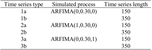
We simulate time series according to the ARFIMA(p,d,q) model, where ARFIMA stands for Autoregressive Fractionally Integrated Moving Average. We use the fracdiff R package [18] to simulate 2 000 time series according to each of the types stated in Table 1. The simulations are performed with zero mean and standard deviation of one.

Time series type Simulated process Time series length

1a ARFIMA(0,0.30,0) 150

1b 350

2a ARFIMA(1,0.30,0) 150

2b 350

3a ARFIMA(0,0.30,1) 150

3b 350

Table 1: Types of time series simulated in the present study

Figure 1: Mean (µ), standard deviation (σ) and Hurst parameter (H) estimates for the deseasonalized monthly time series of streamflow. The vertical red dashed line denotes the median value of the estimates

2.2

Forecasting methods

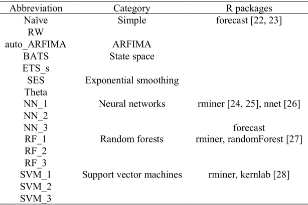
We use the 16 forecasting methods briefly presented in Table 2. The Naïve, RW and auto_ARFIMA forecasting methods serve as benchmarks within our methodological approach, since the former two methods are the simplest ones and the latter is expected to perform better than the rest when applied to ARFIMA processes. The code for the implementation of the forecasting methods can be found in the Supplementary material.

Abbreviation Category R packages

Naïve Simple forecast [22, 23]

RW

auto_ARFIMA ARFIMA

BATS State space

ETS_s

SES Exponential smoothing Theta

NN_1 Neural networks rminer [24, 25], nnet [26] NN_2

NN_3 forecast

RF_1 Random forests rminer, randomForest [27] RF_2

RF_3

SVM_1 Support vector machines rminer, kernlab [28] SVM_2

SVM_3

Table 2: Forecasting methods used in the present study

2.3

Methodology outline

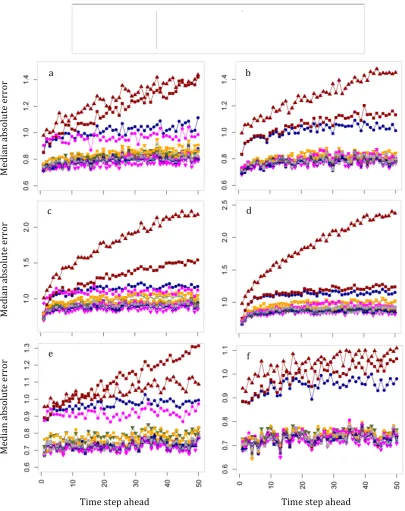
fitting set and make predictions corresponding to the test set using the recursive multi-step ahead forecasting method. Next, we calculate the errors and the absolute errors at each time step of the forecast horizon. We carry out a statistical analysis on the formed data sets and we present the results accordingly. We assess the performance of the forecasting methods by comparing it with the performance of the benchmarks, as well as by comparing the median absolute errors computed at each time step of the forecast horizon with the standard deviation of the time series (available in Section 2.1). The latter comparison is mostly meaningful for the simulated time series, since the median absolute errors for the real-world time series are expected to be more affected by the results of specific time series. The results of the comparative case study are also presented in a qualitative form, to facilitate the detection of systematic patterns.

3

Results and discussion

3.1

Simulation experiments

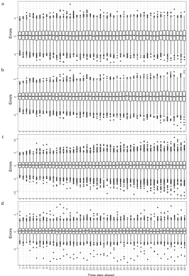
In Section 3.1 we present a representative part of the results of the simulation experiments to support our generalized findings. In more detail, in Figure 2 we present the errors computed at each time step of the forecast horizon within the SE_1a simulation experiment for four forecasting methods producing different error evolution patterns to each other. In fact, we observe that the error evolution can differ to a great extent from the one forecasting method to the other. However, all the error boxplots tend to be approximately symmetric around zero. At the first few time steps ahead we observe an apparent increase of the interquartile range values. This increase is followed by a stabilization of the error histograms for most of the forecasting methods (e.g. Naïve and NN_3). On the contrary, when using the RW and ETS_s forecasting methods the errors seem to keep increasing until the last time step of the forecast horizon. Furthermore, the outliers are more frequent and lay farther from the median values when using specific forecasting methods (e.g. NN_3). This form of instability should also be considered when choosing a forecasting method.

a

b

c

d

Figure 3: Median absolute errors computed at each time step of the forecast horizon within the (a) SE_1a, (b) SE_1b, (c) SE_2a, (d) SE_2b, (e) SE_3a and (f) SE_3b simulation experiments

M

edia

n

ab

sol

ute

e

rr

or

M

edia

n

ab

sol

ute

e

rr

or

M

edia

n

ab

sol

ute

e

rr

or

Time step ahead Time step ahead

e _f

d c

3.2

Comparative case study

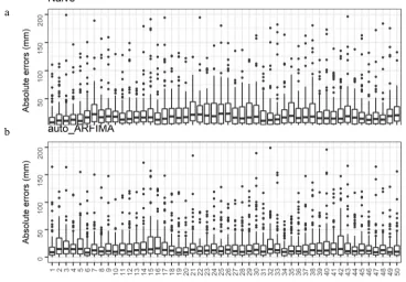
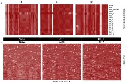
Here as well, the limitations accompanying time series forecasting are highly perceivable. In Figure 4 we present the absolute errors computed at each step of the forecast horizon within the comparative case study for the Naïve and auto_ARFIMA forecasting methods, which could be examined alongside with the standard deviation of the used time series (see Figure 1). We observe that the errors can be large, while auto_ARFIMA and BATS exhibit a very close performance, in average better than the rest of the forecasting methods. Furthermore, in Figure 5 we present a qualitative comparison of the absolute errors computed at each step of the forecast horizon for three examined time series, as well as for three forecasting methods. The relative magnitude of the absolute errors seems to strongly depend on the case examined. Therefore, although some forecasting methods are more likely to produce more accurate forecasts than others and the errors are more likely to be smaller at the first few time steps of the forecast horizon than they are at the next time steps, within a specific single-case study the largest (or the smallest) absolute errors can result from the implementation of any forecasting method at any time step of the forecast horizon.

Figure 4: Absolute errors computed at each time step of the forecast horizon within the comparative case study for a) Naïve and (b) auto_ARFIMA. Outliers larger than 200 mm have been removed

a

Figure 5: Heatmaps for the comparison of the absolute errors computed at each time step of the forecast horizon (a) within three single-case studies, (b) across the 92 examined cases when using Naïve, BATS and

RF_1. The values are scaled in the row direction and the darker the colour the better the forecasts

4

Conclusions

We examine the error evolution in multi-step ahead forecasting using the recursive technique by comparing the performance of 16 forecasting methods on 12 000 simulated time series. Additionally, we conduct a comparative case study using 92 monthly time series of streamflow. Our findings indicate that the error evolution can differ to a great extent from the one forecasting method to the other. This specific information could be used to decide on a forecasting method, since some methods have been proven more useful than others. It could also be used for the proper modelling of the errors, which is still an open challenge for the hydrological community.

Supplementary material

The analyses and visualizations have been performed in R Programming Language [29] by mainly using the contributed R packages forecast [22, 23], fracdiff [18], ggplot2 [30], HKprocess [20], kernlab [28], nnet [26], randomForest [27] and rminer [24, 25]. We provide the code for the implementation of the forecasting methods [31].

a

Fo

rec

asti

ng

m

eth

od

b

Naïve BATS RF_1

T

im

e

ser

ies

Acknowledgements

We thank an anonymous reviewer, whose comments have led to the improvement of the paper.

References

[1] G. Bontempi, S.B. Taieb, Y.A. Le Borgne, Machine learning strategies for time series forecasting, in: M.A. Aufaure, E. Zimányi (Eds.), Business Intelligence, Springer Berlin Heidelberg, 2013, pp 62–77. doi:10.1007/978-3-642-36318-4_3.

[2] S.B. Taieb, G. Bontempi, A.F. Atiya, A. Sorjamaa, A review and comparison of strategies for multi-step ahead time series forecasting based on the NN5 forecasting competition, Expert Syst. Appl. 39 (2012) 7067–7083. doi:10.1016/j.eswa.2012.01.039.

[3] M.S. Khan, P. Coulibaly, Application of support vector machine in lake water level prediction, J. Hydrol. Eng. 11 (2006) 199–205. doi:10.1061/(ASCE)1084-0699(2006)11:3(199).

[4] G.A. Papacharalampous, H. Tyralis, D. Koutsoyiannis, Forecasting of geophysical processes using stochastic and machine learning algorithms. European Water 59 (2017) 161–168.

[5] C.T. Cheng, J.X. Xie, K.W. Chau, M. Layeghifard, A new indirect multi-step-ahead prediction model for a long-term hydrologic prediction, J. Hydrol. 361 (2008) 118–130. doi:10.1016/j.jhydrol.2008.07.040.

[6] P. Coulibaly, F. Anctil, B. Bobee, Daily reservoir inflow forecasting using artificial neural networks with stopped training approach, J. Hydrol. 230 (2000) 244–257. doi:10.1016/S0022-1694(00)00214-6.

[7] M. Valipour, M.E. Banihabib, S.M.R. Behbahani, Comparison of the ARMA, ARIMA, and the autoregressive artificial neural network models in forecasting the monthly inflow of Dez dam reservoir, J. Hydrol. 476 (2013) 433–441. doi:10.1016/j.jhydrol.2012.11.017.

[8] R. Krzysztofowicz, The case for probabilistic forecasting in hydrology, J. Hydrol. 249 (2001) 2–9. doi:10.1016/S0022-1694(01)00420-6.

[9] T. Zhao, X. Cai, D. Yang, Effect of streamflow forecast uncertainty on real-time reservoir operation, Adv. Water Resour. 34 (2011) 495–504. doi:10.1016/j.advwatres.2011.01.004.

[10] S. Makridakis, M. Hibon, E. Lusk, M. Belhadjali, Confidence intervals: An empirical investigation of the series in the M-competition, Int. J. Forecasting 3 (1987) 489–508. doi:10.1016/0169-2070(87)90045-8.

[11] D. Koutsoyiannis, A random walk on water, Hydrol. Earth Syst. Sc. 14 (2010) 585–601. doi:10.5194/hess-14-585-2010.

[12] A. Montanari, D. Koutsoyiannis, A blueprint for process-based modeling of uncertain hydrological systems, Water Resour. Res. 48 (2012). doi:10.1029/2011WR011412.

[13] A.E. Sikorska, A. Montanari, D. Koutsoyiannis, Estimating the uncertainty of hydrological predictions through data-driven resampling techniques, J Hydrol. Eng. 20 (2014). doi:10.1061/(ASCE)HE.1943-5584.0000926.

[14] H. Tyralis, D. Koutsoyiannis, A Bayesian statistical model for deriving the predictive distribution of hydroclimatic variables, Clim. Dynam. 42 (2014) 2867–2883. doi:10.1007/s00382-013-1804-y. [15] H. Tyralis, D. Koutsoyiannis, On the prediction of persistent processes using the output of

deterministic models, Hydrolog. Sci. J. 62 (2017) 2083–2102. doi:10.1080/02626667.2017.1361535.

[18] C. Fraley, F. Leisch, M. Maechler, V. Reisen, A. Lemonte, fracdiff: Fractionally differenced ARIMA aka ARFIMA(p,d,q) models. R package version 1.4-2 (2012). https://CRAN.R-project.org/package=fracdiff.

[19] M.C. Peel, F.H.S. Chiew, A.W. Western, T.A. McMahon, Extension of unimpaired monthly streamflow data and regionalisation of parameter values to estimate streamflow in ungauged catchments. Report prepared for the National Land and Water Resources Audit, 2000.

[20] H. Tyralis, HKprocess: Hurst-Kolmogorov Process, R package version 0.0-2 (2016). https://CRAN.R-project.org/package=HKprocess.

[21] H. Tyralis, D. Koutsoyiannis, Simultaneous estimation of the parameters of the Hurst-Kolmogorov stochastic process, Stoch. Env. Res. Risk. 25 (2011) 21–33. doi:10.1007/s00477-010-0408-x. [22] R.J. Hyndman, M. O'Hara-Wild, C. Bergmeir, S. Razbash, E. Wang, forecast: Forecasting

functions for time series and linear models, R package version 8.0 (2017). https://CRAN.R-project.org/package=forecast.

[23] R.J. Hyndman, Y. Khandakar, Automatic time series forecasting: the forecast package for R, J. Stat. Softw. 27 (2008) 1–22. doi:10.18637/jss.v027.i03.

[24] P. Cortez, Data mining with neural networks and support vector machines using the R/rminer tool, in: P. Perner (Eds.), Advances in Data Mining, Applications and Theoretical Aspects, Springer Berlin Heidelberg, 2010, pp 572–583. doi:10.1007/978-3-642-14400-4_44.

[25] P. Cortez, rminer: Data Mining Classification and Regression Methods, R package version 1.4.2 (2016). https://cran.r-project.org/web/packages/rminer/index.html.

[26] W.N. Venables, B.D. Ripley, Modern Applied Statistics with S, fourth edition, New-York: Springer-Verlag, 2002. doi:10.1007/978-0-387-21706-2.

[27] A. Liaw, M. Wiener, Classification and regression by randomForest, R News 2 (2002) 18–22. [28] A. Karatzoglou, A. Smola, K. Hornik, A. Zeileis, kernlab - An S4 Package for Kernel Methods in

R, J. Stat. Softw. 11 (2004) 1–20.

[29] R Core Team, R: A language and environment for statistical computing, R Foundation for Statistical Computing, Vienna, Austria, 2017. https://www.R-project.org/.

[30] H. Wickham, ggplot2: elegant graphics for data analysis, second ed., Springer International Publishing, Switzerland, 2016. doi:10.1007/978-3-319-24277-4.