Rare event analysis using the Limited Relative Error algorithm for OMNeT++ simulations

Volume 56, 2018, Pages 93–101

Proceedings of the 5th International OMNeT++ Community Summit

Rare event analysis using the Limited Relative Error

algorithm for OMNeT++ simulations

Sebastian Lindner, Raphael Elsner, Phuong Nga Tran, and Andreas Timm-Giel

Institute of Communication Networks (ComNets)

Hamburg University of Technology (TUHH)

Hamburg, Germany

{sebastian.lindner, raphael.elsner, phuong.tran, timm-giel}@tuhh.de

Abstract

The Limited Relative Error algorithm is an alternative statistical method for data evaluation. Through online result analysis it continuously requests more samples until it deems the evaluation confident enough. With this it allows researchers to hand over the control of simulation time to the algorithm, and through a-priori configuration the target result resolution is set so that arbitrarily rare events can be investigated. We provide a new description of the method as well as a stand-alone implementation and an integration of the algorithm into the OMNeT++ simulator.

1

Introduction

A crucial part of stochastic simulation is the statistical evaluation of the result data. To make an objective statement about the accuracy of one’s results, the quantity of data or equivalently the simulation time must be taken into account.

The popularBatch Means evaluation method is, according to [1], deficient as it attempts to eliminate correlation by forming “quasi-independent, quasi-normally distributed batch-random variables”. The replication method eliminates correlation through the repetition of the same scenario with varying random number generator seeds. This suffers from having to eliminate the warmup period of each repetition. Both methods have the disadvantage of having to estimate the required simulation time a-priori. Akaroa2, presented in [2], aims to solve this problem by running distributed, statistically independent simulations on isolated hosts or processes, which report their progress to a central analyser, which in turn requests the hosts to stop once it deems the results confident enough.

The lesser-known Limited Relative Error (LRE) algorithm will be reviewed in this paper, which estimates an unknown cumulative distribution function (CDF) function corresponding to the observations made during simulation. The algorithm does an online analysis of the simulation resultsduring simulation, and so controls the simulation length until the relative error dhas been decreased past the target errord≤dmax by requesting more observations. d

In contrast to Akaroa2, the distribution of a statistic in question is evaluated, as opposed to the mean. Therefore LRE tackles a different problem and is especially suitable for applications in reliability analysis, where the user knows a-priori that a system should not exceed some performance boundaries; say Voice over IP (VoIP) applications should not experience packet delays exceeding 150 ms, and the researcher aims to find out how likely it is to violate this boundary. On the other hand, analysis methods for mean values based on confidence intervals are better suited to establish a picture of the range of some statistic.

In certain applications, very rare events want to be investigated. Very long simulation runs are required to obtain a sufficient number of observations, and time constraints make this a difficult problem, especially if emulators instead of simulators are used. Estimating the required simulation time to obtain a sufficient number of observations is especially difficult in this case. The paper is organized as follows. In Section2a brief history of the LRE algorithm is given. Section3 attempts to describe the algorithm in detail. Section 4gives a quick example of the application of the algorithm on work conducted using the OMNeT++ simulator, and Section5

concludes the document.

2

Related Work

The LRE algorithm evolved over the span of more than a decade. In 1984 Schreiber published the first version in [3], where a sequence of observations was assumed to be independent. In 1988, Schreiber published an extension in [4], where the correlation of the observations was considered. In 1996, Schreiber and G¨org published the third iteration of the algorithm in [1], which is further discussed in G¨org’s habilitation in [5]. In [6] it is evaluated for reliability, while [7] gives an analysis of the algorithm from the perspective of sojourn times, where a disadvan-tage of inaccurate confidence is highlighted in certain cases, as well as doubt raised about the modelling of samples through amemoryless Markov chain, which may be unrealistic. However the advantage of not having to estimate the simulation time may outweigh this disadvantage.

LRE-III is a simplified version that requires the observations to bediscrete, while the earlier versions were able to also cope with continuous and mixed continuous-discrete observations.

3

Limited Relative Error algorithm

This section covers the functionality of the LRE algorithm as taken from the various publications by the authors in [1], [3], [4] and [5].

3.1

Assumptions and Goals

Given a chronological sequence of observations (α1, α2, . . . , αn) that stem from a random

pro-cessX, the following assumptions are typically made for the field of communication networks, from [5]: (a) the samples are correlated, (b) the random process X is stationary; that is, a time-independent CDF FX(x) is associated with the sample sequence and (c) the type of the

random process is unknown; that is, all ofFX(x) as well as correlations are not known a-priori.

The goal of the LRE algorithm is therefore to (a) find FeX(x) as an approximation of the

unknownFX(x), (b) make statements about the correlation of the sample sequence, (c)

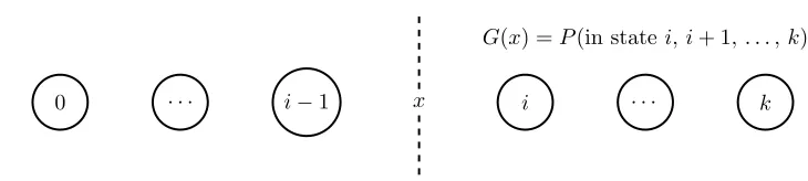
0 . . . i−1 x i . . . k G(x) =P(in statei, i+ 1, . . . , k)

Figure 1: Graphical visualization ofG(x) in Equation1. iis the first state that corresponds to a sample whose value is larger thanx.

3.2

Complementary cumulative distribution function

We can order our observations into (α01, α02, . . . , αn0) with αi0 ≤ α0i+1. For every x we can

now easily find aleft andright subvector containing only smaller and equal, or greater values. (α0₁, α₂0, . . . , α0_n) corresponds to a discrete (k+ 1)-state Markov chain, where each state cor-responds to observing a particular sample, and state k corresponds to the observation of the largest observed sample.

For this Markov chain, the complementary cumulative distribution function (CCDF) can be found as

G(x) =Gi=P(X > x) = k X

j=i

Pj fori−1≤x < i, i= 1,2, . . . , k

withG0= 1 and Gk+1= 0

(1)

G(x) in Equation 1 corresponds to the probability of being in any state that corresponds to the random variableX taking on a value larger thanx, which corresponds to the CCDF, as shown in Figure1.

3.3

Markov Chains

For every positionxin the (k+ 1)-state Markov chain, a 2-state Markov chain as in Figure 2

can be obtained, where the first state corresponds to the random variableX taking on values X≤xand the second state toX > x.

The transition probabilitiesp0(x), p1(x) can be found as follows:

p0(x) =

1 F(x)

i−1 X r=0 Pr k X j=i

prj fori−1≤x < i, i= 1,2, . . . , k

p1(x) =

1 G(x)

k X r=i Pr i−1 X j=0

prj fori−1≤x < i, i= 1,2, . . . , k

(2)

3.4

Local Correlation Coefficient

The covariance normalized by the standard deviation is thecorrelation coefficient ρ:

ρXY =Corr(X, Y) =

Cov(X, Y) σXσY

Figure 2: A local x-based 2-state Markov chain obtained from a (k+ 1)-state Markov chain. From [5].

where−1≤ρ≤1.

Whileρconsiders all values of the random variablesX, Y, the local correlation coefficient ρ(x) is a function ofx, and therefore depends on this positionx. Considering 2-state Markov chains, their global correlation coefficientρcorresponds to the local correlation coefficientρ(x) of the underlying (k+ 1)-state Markov chain at the respective positionx.

The local coefficient can be found asρ(x) = 1−[p0(x) +p1(x)], where forp0(x) +p1(x)<1

a positive correlation is found according to [5]. In other words, this means that there is a larger probability that once either state is entered, the process will remain in that state for one or more iterations, than if the state has not been entered. This corresponds to burstiness of for example packet delays, where it is likely to observe more large delays once a single large delay has been observed. With this, the state probabilitiesP0(x), P1(x) for the 2-state Markov chain

of being in stateS0(x), S1(x) respectively are

P0(x) =

p1(x)

1−ρ(x)

P1(x) = 1−P0(x) =

p0(x)

1−ρ(x)

(4)

3.5

Procedure

The algorithm aims to determine – through simulation – the CCDFG(x) of a (k+ 1)-state Markov chain wherekis given a-priori, and where transition probabilitiespji arenot known.

To do this, we count how many times each state ihas been entered after n transitions in the chain. We save this number in the counter variablehi, from which we can find the state

frequency

vi= k X

j=i

hj fori= 0,1, . . . , k with v0=n (5)

that tells us how many times the right stateS1(x) with i−1 ≤x < i of the 2-state Markov

chain has been entered – for reference see Figure2. ri=n−vi handles the left stateS0(x) and

is implicitly counted.

Thetransition frequency ci, i= 1,2, . . . , k counts how many times the transitionS1(x)→

counterpartsri =n−vi andai≈ci belong to the equivalentx-based 2-state Markov chain.

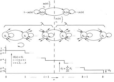
An overview is given in Figure3.

Figure 3: An overview of the transformation from a (k+ 1)-state to a 2-state Markov chain, as well as countersai, ci, ri, viand the association withGi. From [5].

Next, after having measuredvi, cifromnsamples, thelarge sample conditions are checked:

n≥103require “many” samples; makes sure the transient phase has been left

(ri, vi)≥102at least 100 samples left and right of state i

ci, ai≥10 at least 10 transitions from statei

vi−ci≥10 have at least 10 more visits than leaves (sometimes remain in state)

and if met, we can determine (a) the measured CCDF Ge(x) = Gei = v_ni, (b) the

measured state average α_e = _n1Pk_i=1vi, (c) the measured local correlation coefficient

e

ρ(x) = _eρi = 1− ci/vi

1−vi/n, (d) the corresponding correlation factor fcf(x) = cffi =

1+_eρi

1−_eρi and

(e) the relative errordG(x) =di=σG(x)/Ge(x) = r

_1−v

i/n

vi ·fcfi

.

HereσG(x) is the standard deviation ofP1(x) in the 2-state Markov chain, which was found

in [7] and [8] to be normally distributed. As the transitions are counted in ci, not only the

local correlation coefficient ρ_e(x) but also the relative error dG(x) as a function of ρ_e(x) can

error condition di ≤ dmax is met, where dmax is an a-priori maximum error. The standard

deviation σG(x) gives an absolute error, which is made relative to the probability of being

in state ≥ i of the Markov chain by dividing with the value of the CCDF at the respective positionGe(x). The correlation coefficient becomes large for a large, positive correlation, and

so increases the relative error. A large correlation corresponds to many transitions from a state to itself (e.g. burst errors resulting in a long sojourn time in the large-error-state), and so the algorithm demands more observations in this case to ensure that the transition probabilities

between states are accurately modelled.

3.6

Executing the algorithm

Parameters for a simulation supervised by LRE aredmax, xmin, xmax, xstep. The sequence of

samplesx1, x2, . . . , xn is mapped to the (k+ 1)-state Markov chain, and nis increased until

di≤dmaxfor alli. At runtime an indexscorresponds to that state in the Markov chain whose

errords shall be checked next, and it is initialized ats= 1.

Algorithm 1LRE Algorithm; adapted from [5]

1: procedurelre simulation(maximum errordmax, bounds of evaluation rangexmin, xmax,

interval sizexstep)

2: k= (xmax−xmin)/xstep .largest state index

3: fori= 0, . . . , kdo

4: hi= 0;ci= 0 .initialize counters

5: x= 0; n= 0;s= 1

6: whiles6=kdo . iterate through states 1. . . k

7: ω=x . remember old value

8: generate new observationx

9: increment counterhx

10: increment number of samplesn

11: if x < ωthen . transition to left ofω

12: fori=x+ 1 toω do

13: incrementci .state transition to smaller value

14: calculateρ_esand relative errords

15: if ds≤dmax then .target error reached?

16: increment s . go to next state

17: fori= 1, . . . , kdo

18: calculate sum frequenciesvi from Equation5 19: calculate result valuesGei,ρei, di

4

Application

A standalone LRE implementation is available on GitHub in [9], which is also used for our OMNeT++ integration available in [10]. The novel LRE OMNeT++ entity subscribes to a

Configuration of the entity is done through setting NED parameters. The output corre-sponds to the measured probability of the CCDF at all x-positions, as well as the relative errord(x), local correlation coefficient ρ(x), standard deviation σ(x), number of samples and transitions per staten(x), t(x).

4.1

Example

An example use case is included in the implementation in [10]. A simple network with one sender and one receiver is modelled. The sender draws the time it waits until sending the next packet from an exponential distribution with a mean of 150 ms. We quantise the packet interarrival times measured at the receiver into intervals of size xstep = 100 ms and observe

the rangexmin = 0 ms ≤x ≤xmax = 1000 ms. We repeat the LRE runs for the maximum

errorsdmax∈[0.01,0.015,0.02,0.025,0.03, 0.035,0.04,0.045, 0.05] to see how the target error

affects the required number of observations.

This simple approach is chosen so that it is easily understood and imitated by new users of the LRE method. As all code required to replicate the exact results is part of the open-source code release in [10], it shall provide easy access to understanding how the LRE method is used in OMNeT++.

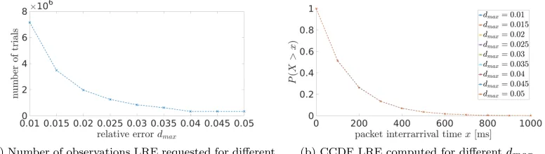
(a) Number of observations LRE requested for different

dmax.

(b) CCDF LRE computed for differentdmax.

Figure 4: Number of observations requested and CCDF measured by the LRE for OMNeT++ integration of packet interarrival times measured at the receiver.

Figure4ashows that the number of observations increases strongly as the maximum allowed error dmax decreases. In our test case, when dmax = 1 % then the number of observations

is 27 times larger than the number of observations for dmax = 5 %. Figure 4b shows the

corresponding CCDF, where the three cases of dmax correspond to measured probabilities

that differ in the range of 0.1 %. The largest packet interrarival times occur at probability P(X >1000 ms)≈10−3.

We can conclude that the LRE algorithm successfully controls the number of observations it requires and so the simulation time. When a more rigid analysis is required,dmaxis set to a

5

Summary, Conclusion, and Outlook

In this paper we have demonstrated a lesser-known but useful statistical method for result evaluation that is capable of deciding when a simulation shall end automatically, ensuring that an a-priori target confidence level is met. The LRE algorithm can be configured so that the intended resolution of some statistic is measured – so if the user is interested in rare events, then the target resolution is easily configured, and the algorithm will ensure that a confident statement can be made afterwards.

We have provided a new description of the LRE algorithm which dates back to the eighties and nineties. An OMNeT++ network module is implemented that provides the algorithm func-tionality to the simulator. Through simple network configuration the algorithm is configured, and when the simulation time is unset or set to a very large value, the LRE entity will handle simulation termination when the results have reached the target confidence level. This allows the easy analysis of arbitrarily rare event statistics in OMNeT++. Events that occur with a very small probability can not be investigated more quickly as the simulation time may still be prohibitively long; so far the gain is the automatic on-line evaluation and termination when the target confidence is met. The LRE method was combined in [11] with the RESTART method, first published in [12], to significantly decrease the required simulation time. An implementation of this in OMNeT++ could prove useful to many researchers.

We have made available both the standalone implemenation in [9] as well as the OMNeT++ integration in [10]. The network model that generates the data shown in this paper is part of the release in [10].

References

[1] F. Schreiber and C. G¨org, “Stochastic simulation: A simplified LRE-algorithm for discrete random sequences,”AE ¨U - International Journal of Electronics and Communications, vol. 50, no. 4, pp. 233–239, 1996.

[2] G. C. Ewing, K. Pawlikowski, and D. McNickle, “Akaroa2: Exploiting network computing by distributing stochastic simulation,” in Proceedings of the European Simulation Multiconference ESM’99. International Society for Computer Simulation, 1999, pp. 175–181.

[3] F. Schreiber, “Time efficient simulation the lre-algorithm for producing empirical distribution functions with limited relative error,”AE ¨U - International Journal of Electronics and Communi-cations, vol. 2, no. 38, pp. 93–98, 1984.

[4] ——, “Effective control of simulation runs by a new evaluation algorithm for correlated random sequences,”AE ¨U - International Journal of Electronics and Communications, vol. 42, no. 6, pp. 347–354, 1988.

[5] C. G¨org, “Verkehrstheoretische Modelle und Stochastische Simulationstechniken zur Leistungs-analyse von Kommunikationsnetzen,” Habilitation, RWTH Aachen, Germany, 1997.

[6] K. Below, L. Battaglia, and U. Killat, “RESTART/LRE Simulation - the reliability issue,” Ham-burg University of Technology, Tech. Rep., 1999.

[7] N. T. M¨uller, “An analysis of the LRE-algorithm using sojourn times,” in Proceedings of the 14th European Simulation Multiconference on Simulation and Modelling (ESM 2000), R. van Lan-deghem, Ed. SCS Europe, 2000, pp. 149–153.

[8] F. Schreiber, “Reliable evaluation of simulation output data: A simplified formula basis for the LRE-algorithm,” inProceedings of the MMB ’99. VDE Verlag Berlin, 1999, pp. 137–152. [9] “LRE implementation.” [Online]. Available: https://doi.org/10.5281/zenodo.1312970

[11] C. G¨org and F. Schreiber, “The RESTART/LRE method for rare event simulation,” inProceedings of the 1996 Winter Simulation Conference, J. M. Charnes, D. J. Morrice, D. T. Brunner, and J. J. Swain, Eds., 1996, pp. 390–397.