Volume 57, 2018, Pages 164–180
LPAR-22. 22nd International Conference on Logic for Programming, Artificial Intelligence and Reasoning
A Verified Efficient Implementation of
the LLL Basis Reduction Algorithm
Ralph Bottesch, Max W. Haslbeck, and Ren´
e Thiemann
University of Innsbruck, Austria
Abstract
The LLL basis reduction algorithm was the first polynomial-time algorithm to compute a reduced basis of a given lattice, and hence also a short vector in the lattice. It thereby approximately solves an NP-hard problem. The algorithm has several applications in number theory, computer algebra and cryptography.
Recently, the first mechanized soundness proof of the LLL algorithm has been developed in Isabelle/HOL. However, this proof did not include a formal statement of the algorithm’s complexity. Furthermore, the resulting implementation was inefficient in practice.
We address both of these shortcomings in this paper. First, we prove the correctness of a more efficient implementation of the LLL algorithm that uses only integer computations. Second, we formally prove statements on the polynomial running-time.
1
Introduction
The LLL basis reduction algorithm, originally introduced by (and named after) Lenstra, Lenstra and Lov´asz [11], is a remarkable algorithm with numerous applications. The algorithm computes an approximate solution to the following problem:
Shortest Vector Problem (SVP): Given a linearly independent set of m vectors,
f0, . . . , fm−1∈Zn, which form a basis of the correspondinglattice (the set of vectors that can be written as linear combinations of thefi, with integer coefficients), compute a non-zero lattice
vector that has the smallest-possible norm.
This problem plays an important role in number theory and cryptography [14]. It is NP-hard to solve exactly in general [13], but, given any basis of a latticeLas input, the LLL algorithm computes, in polynomial time, a basis ofL that isreduced w.r.t. α, which implies, among other things, that the shortest vector in the basis is at mostαm2−1 times larger than the shortest
non-zero vector in the lattice. Here,α > 4
3 is a parameter of the algorithm that also appears in the running time.
is important not mainly because the correctness of the algorithms themselves might be in doubt, but because such implementations can be composed into large reliable programs, of which every part has been formally proved to work as intended.
Our first contribution is to modify the verified implementation of the LLL algorithm from [5] so as to make it considerably faster. Although both the input and the output of instances of
SVPare sets of integer-valued vectors, the original formalization followed a particular textbook
version of the algorithm, that makes extensive use of computations on rational numbers. We determined via tests that gcd computations, which are necessary in order to reduce fractions, accounted for at least 83 % of the running time of that implementation on each input. In order to improve on this, we followed [7,18] to obtain a fully verified, integer-only implementation of the LLL algorithm, thus eliminating the need for the use of rational numbers altogether.
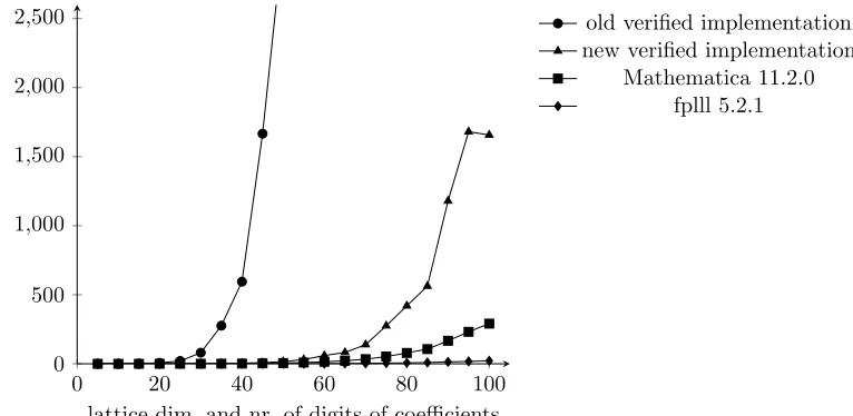
The corresponding generated Haskell code now runs in time comparable to that of the LLL implementation in some commercial software packages for mathematical computations, such as Mathematica (see Figure1). Specifically, in numerical experiments, our new implementation was, at worst, about 7x slower than Mathematica; usually the two were much closer in speed. This means that, in addition to having the advantage of being formally verified, our implementation is now usable in practice. By contrast, on lattices of dimension n ≥ 30, the old verified implementation is at least 3ntimes slower than the new one. However, it should be noted that specialized floating-point implementations of LLL like fplll [19] are still orders of magnitude faster than either our new implementation or the one in Mathematica.
0 20 40 60 80 100
0 500 1,000 1,500 2,000 2,500
lattice dim. and nr. of digits of coefficients
time
in
s
old verified implementation new verified implementation
Mathematica 11.2.0 fplll 5.2.1
Figure 1: A comparison of the performance of LLL implementations on lattices obtained from instances of polynomial factorization. The verified implementations were run with α = 3
2. Mathematica and fplll used their default values forα, which are even closer to 4
3, resulting in slightly better approximations of shortest vectors.
using a number of bits that is polynomial in the size of the input. The two main Isabelle lemmas expressing these facts are the following:
• lemmareduce basis cost expanded:
assumesLg=natdlog(of rat(4 ·α/ (4+α))) Ae andA=Max{kvk2|v. v∈set fs}
showscost(reduce basis cost fs)≤49·m3 ·n·Lg (* illustrative bound *)
The functionreduce basis costis an extended version ofreduce basis (which implements the (integer) LLL algorithm). The extended function returns the result of the original function, together with the number of arithmetic operations required to compute it. The above lemma then gives a polynomial upper bound on this number of required operations, whereAis the maximum squared norm of the input vectors, andLg is the logarithm ofA with base 4+4αα (which is>1 whenα > 43). The above bound is a simplified version of the finer bound from the code, and only serves to illustrate the fact that it is polynomial.
• lemmacombined size bound integer: assumes... andM=Max{|fs ! i $ j| |i j. i<m∧j<n}
andx∈... (* description of numbers during run of algorithm *)
showslog 2|x| ≤(6 +6·m)·log 2(M·n) +m+log 2 m
The second lemma combines the size bounds for all numbers computed by the algorithm throughout its run. Here,M is the maximum absolute value occurring in the inputfs.
Together, the two lemmas imply the polynomial complexity of our implementation of the LLL algorithm, since each arithmetic operation can be computed in polynomial time, and only polynomially many such operations are executed.
The two contributions amount to a considerable expansion of the original project of [5], with the code base having roughly doubled. The new proofs are available in the Archive of Formal Proofs (AFP) for Isabelle 2018, entry LLL Basis Reduction [1]. All definitions and lemmas found in this paper are also links which lead to an HTML version of the corresponding Isabelle theory file. The code referenced here can be found in the follow-ing theories: Gram Schmidt Int.thy, LLL Number Bounds.thy, LLL Integer Equations.thy,
LLL Mu Integer Impl.thy, and LLL Mu Integer Impl Complexity.thy. We provide further
installation instructions for the formalization athttp://cl-informatik.uibk.ac.at/isafor/ experiments/lll. This website also contains experimental data, such as the input matrices, the experimental setup, and the Haskell code of the old and the new verified LLL implementation.
The remaining sections are organized as follows: We first recall the existing formalization in Section2. In Section3we discuss the details of implementing and proving the correctness of the integer LLL algorithm in Isabelle. We illustrate the formal proof of the bound on the number of arithmetic operations in Section4, and present the bounds on the size of the numbers in Section 5. We discuss the technicalities of using Cramer’s lemma in Isabelle in Section 6. Finally, we conclude in Section7.
2
Preliminaries
Interactive theorem proving
Our tool of choice for the formalization of proofs is Isabelle/HOL. We assume familiarity with it, and refer the reader to [16] for a quick introduction, but nevertheless we briefly review some Isabelle notation, which should make most of the code segments accessible to readers familiar only with standard mathematical notation.
All terms in Isabelle must have a well-defined type, specified with a double-colon: term :: type. Type variables have a 0 sign before the identifier. The type of a function with domainA and
rangeBis specified asA⇒B. Each of the base typesnat,int andratcorresponds to the number set suggested by its name. Access to an element of a vector, list, or array is denoted, respectively, by$,!, !!. For example, iffs is of typeint vec list, the type of lists of vectors of integers, then fs ! i $ j denotes thej-th component of thei-th vector in the list. In the text, we will often use more common mathematical notation instead of Isabelle notation. For example, we would writefi rather thanfs ! i. The syntax for function application in Isabelle isfunc arg1 arg2 ...;
terms are separated by white spaces, andfunc can be either the name of a function or a lambda expression. Note that some terms that we index with subscripts in the in-text mathematical notation are defined as functions in the Isabelle code (for exampleµi,j stands formu i j).
The Formalized LLL Algorithm
In this section we briefly review the existing Isabelle/HOL formalization of the LLL algorithm [5], focusing only on the process of formally verifying its correctness; for an explanation of the algorithm itself, we refer to [25] or [14].
The algorithm to be formalized is given as pseudo-code in Algorithm1. Here,bxe=bx+12cis the integer nearest tox, the inner product of vectorsuandv is denoted byu•v, andkuk2=u•u
is the squared Euclidean norm ofu. The valuesgi andµi,j are defined as follows, with f always
referring to the current values off in Algorithm 1:
gi=fi− X
j<i
µi,j·gj µi,j:=
1 ifj=i 0 ifj > i
fi•gj
kgjk2 ifj < i.
The vectors g are the so-called Gram–Schmidt orthogonalization (GSO) vectors and the recursive definitions of g and µ describe the Gram–Schmidt orthogonalization procedure. If f0, . . . , fm−1 are a list of linearly independent vectors inRn orQn, then g0, . . . , gm−1 are an orthogonal basis for the space spanned by f0, . . . , fm−1. This procedure has already been
Algorithm 1: The LLL basis reduction algorithm, verified version
Input: A list of linearly independent vectors f0, . . . , fm−1∈Zn andα > 43
Output: A basis for the same lattice asf0, . . . , fm−1, that is reduced w.r.t.α
1 i:= 0
2 while i < mdo
3 forj =i−1, . . . ,0 do 4 fi:=fi− bµi,je ·fj
5 if i >0∧ kgi−1k2> α· kgik2then
6 (i, fi−1, fi) := (i−1, fi, fi−1)
else
7 i:=i+ 1
8 returnf0, . . . , fm−1
The overall approach to formalizing the rest of Algorithm1is as follows (although we note that the presentation here hides some refinements). First, the algorithm is encoded in several functions (see the explanations following the code). From here onward, throughout the rest of the paper, we present Isabelle code residing in a context that fixes the approximation factorα, the dimensionsnandm, and the basisfsinit of the initial (input) lattice.
definitionbasis reduction step :: (nat ×int vec list)⇒(nat×int vec list)where
basis reduction step(i, fs) =... (* implementation of lines 3−7 *)
partial function(tailrec)basis reduction main ::(nat×int vec list)⇒int vec list where basis reduction main(i, fs) = (
ifi<m
thenbasis reduction main(basis reduction step(i, fs)) elsefs)
definitionreduce basis :: int vec list ⇒int vec list where reduce basis fs=basis reduction main(0, fs)
Some remarks about the above code fragments:
• The body of the while-loop (lines3–7) is modeled by the functionbasis reduction step, the details of which we omit.
• The while-loop itself (line2) is modeled as the partial functionbasis reduction main. Note that the function is not necessarily terminating, since there is no restriction on the validity of inputs (e.g.α= 0 is not ruled out). Putting these assumptions into the context might be possible for proving properties of the LLL algorithm, but would prevent code-generation.
• Finally, the full algorithm is implemented as the functionreduce basis, which starts the loop and then returns the final integer basisf0, . . . , fm−1.
independence. The predicate reduced k fs requires that the current g and µ values of the first k vectors of fs are reduced w.r.t. α, i.e., that µi,j ≤ 12 holds for allj < i < k and that
kgik2≤α· kgi+1k2 holds for alli < k−1.
definitionLLL invariant i fs = ( lin indpt list fs∧
lattice of fs=lattice of fs init∧ length fs=m∧
reduced i fs∧ i≤m)
The key correctness property of the LLL algorithm is then given by the following lemma, which states that the invariant is preserved in the while-loop of Algorithm1(specifically, that if the current state, prior to the execution of an instruction, satisfies the invariant, then so does the resulting state after the instruction). The lemma also states that a measure indicating how far the algorithm is from completing the computation, is decreasing – this is used to prove that the algorithm terminates.
lemmabasis reduction step:
assumesLLL invariant i fs andi<m andbasis reduction step(i, fs) = (i0, fs0) showsLLL invariant i0 fs0
andLLL measure i0 fs0 <LLL measure i fs
Finally, using Lemmabasis reduction step, one can prove the following crucial properties of the LLL algorithm. Again,Ais the maximum squared norm of the initial lattice basisfsinit.
1. The resulting basis is reduced and is a basis for the same lattice as the initial basis. The first element of the reduced basis is an approximation of the shortest vector in the lattice.
lemmashort vector:
assumesv=hd (reduce basis fs)andh∈lattice of fs− {0} showskvk2≤αm−1khk2
2. The algorithm terminates, since theLLL measure is decreasing in each iteration.
3. The number of loop iterations is bounded byLLL measure i fs when invoking the algorithm on inputsi andfs, so reduce basis requires at mostLLL measure i fsmany iterations.
4. LLL measure i fs≤m+ 2·m·m· log(4+4·αα)A
These properties have all been stated and proved in [5]. There, the verified algorithm already contains some optimizations, e.g., thegvectors are incrementally updated wheneverf is changed, instead of computingg from scratch in every iteration. Using the upper bound for theLLL measure, one can derive a total bound ofO(m3·n·logA) arithmetic operations for the LLL algorithm. However, this has not been done formally in [5], nor has a bound on the values offi,
gi andµi,j been formally proved. Especially, the latter property is not at all obvious and it is
3
A Formally Verified Integer Implementation of the LLL
Algorithm
In this section we describe the formalization in Isabelle of a version of the LLL algorithm that uses only integers. As mentioned in the introduction, such an implementation is desirable for efficiency reasons.
To obtain an implementation of the LLL algorithm that uses only integer operations, we modify the Isabelle implementation of this algorithm from [5]. This modification is necessary because in order to perform the essential computations of the LLL algorithm, one needs to keep track of either theµ-matrix or the GSO-vectors corresponding to the (current) set off vectors, neither of which contain integers in general. We therefore replace theµ-matrix by a matrix of integers with a similar meaning.
Given a set of vectorsv1, . . . , vn, entry (i, j) of the correspondingGramian matrix is defined
to be vi•vj. In our case, the vectors vi are the fi. The Gramian determinant then, is the
determinant of the Gramian matrix.
There are multiple ways to define and characterize the Gramian matrix and determinant in Isabelle. From here onward, all of the code we show resides in a context in which thef vectors form a linearly independent set.
definitionGramian matrix fs k= (let M=mat k n (λ(i, j). (fs ! i)$ j)inM ·MT)
lemma assumesk<m
showsGramian matrix fs k=mat k k(λ(i, j). fs ! i•fs ! j)
For brevity of notation, we will denote Gramian determinant fs k bydk ord k, unless we
wish to emphasize that dk is defined as a determinant. Note thatGramian determinant depends
explicitly onfs, whereas this dependency is implicit ford; whenever a quantity depends implicitly onfs, we assume that we are working in a context wherefs is fixed.
definitiond k=det(Gramian matrix fs k)
lemmaGramian determinant: assumesk ≤m
showsd k= (Qj<k.
kgs ! jk2)
Apart from the integer implementation, the Gramian determinant also appears when proving the termination of the LLL algorithm (it is used to defineLLL measure), as well as when proving upper bounds on the numbers that are computed in the course of a run of the algorithm (see Section5).
The most important fact for the integer implementation is given by the following lemma:
lemmaGramian determinant mu ints: assumesj≤i andi<m
showsd(Suc j)· µi j∈Z
Based on this fact we derive a LLL implementation which only tracks the values of ˜µ, where ˜
µi,j:=dj+1µi,j (in the Isabelle source code, ˜µis calleddµ). We can show that the ˜µvalues can
3.1
An Integer Implementation of Gram–Schmidt Orthogonalization
Since the LLL algorithm performs Gram–Schmidt orthogonalization as a subroutine, a full integer-only implementation of the former also requires such an implementation of the latter. For this, we mainly follow [7], where a GSO-algorithm using only operations in an abstract integral domain is given. We made some small simplifications to this algorithm and then formalized in Isabelle most of the proofs from [7].
Algorithm 2: Gram–Schmidt orthogonalization (adapted from [7]) – for ˜µ-values only
Input: A list of linearly independent vectors f0, . . . , fm−1∈Zn
Output: µ˜where ˜µi,j=dj+1µi,j
1 fori= 0, . . . , m−1 do 2 µ˜i,0:=fi•f0
3 forj = 1, . . . , ido 4 σ:= ˜µi,0µ˜j,0
5 forl= 1, . . . , j−1do
6 σ:= (˜µl,lσ+ ˜µi,lµ˜j,l) div ˜µl−1,l−1
7 µ˜i,j:= ˜µj−1,j−1(fi•fj)−σ
8 returnµ˜
The correctness of Algorithm2hinges on two properties: that the calculated ˜µi,jare equal to
dj+1µi,j, and that it is correct to use integer division in line6 of the algorithm (in other words,
that the intermediate values computed at every step of the algorithm are integers). We prove these two statements in Isabelle by starting out with a more abstract version of the algorithm, which we then refine to the one above. Specifically, we first define the relevant quantities
definitionµ˜ i j=d(Suc i)·µi j funσwhere
σ0 i j=0
|σ(Suc l)i j= (d(Suc l)·σl i j+ ˜µi l·µ˜ j l)/ d l
whereσl i j represents the value ofσat thel-th pass through the innermost loop. Note that the type of (the range of) ˜µandσisratand not int, which is why we can use general division (for fields) in the above function definition, rather thandiv. The advantage of letting ˜µandσhave more general types is that we can proceed to prove all of the equations and lemmas from [7] while focusing only on underlying mathematics, without having to worry on non-exact division. For example, from the definition above we can easily show the following characterization:
lemmaσ: assumesl≤m showsσl i j=d l ·(P
k <l. µi k·µj k · kgs ! jk2)
which is needed to prove one of the two statements that are crucial for the correctness of the algorithm:
lemmaσinteger:
We also mention that the proof of Lemma σinteger requires an application of Cramer’s lemma. The difficulties with applying this lemma in Isabelle are described in Section6.
The other ingredient required to prove correctness is to show how ˜µ can be computed in terms ofσ.
lemmaµ:˜ assumesj≤i andi<m showsµ˜ i j=d j·(fs ! i·fs ! j)−σj i j
Having proved the desired properties of the abstract version of the algorithm, we make the connection with an actual implementation that computes the values of ˜µrecursively. Here, the identitiesdj+1 = ˜µj,j and d0 = 1 are also included; they show that the ˜µ-values include the
d-values in particular.
funσZ :: nat⇒nat ⇒nat ⇒intandµ˜Z :: nat⇒nat⇒int where σZ 0 i j= ˜µZ i 0·µ˜Z j 0
|σZ (Suc l)i j= (˜µZ (Suc l) (Suc l)·σZ l i j
+ ˜µZ i(Suc l)·µ˜Z j(Suc l))div µ˜Zl l |µ˜Z i j= (if j=0 then fs ! i·fs ! j
elseµ˜Z (j−1) (j−1)·(fs ! i· fs ! j)−σZ (j−1)i j)
Note that these functions only use integer arithmetic and therefore return a value of type int. We then show that the new functions are equal to the ones defined previously. Here,of intis a function that converts a number of type intinto the corresponding number of typerat. Further note that the indices ofσZ are shifted by 1 with respect to the indices ofσ. This is for the sake of ease of implementation.
lemmaσZ µ: l˜ <j=⇒j≤i=⇒i<m=⇒of int(σZl i j) = σ(Suc l)i j i<m=⇒j≤i=⇒of int(˜µZ i j) = ˜µi j
We then replace the repeated calls of ˜µZby saving already computed values in an array for fast access. Furthermore, we rewriteσZ to be a tail-recursive function, which completes the integer implementation of the algorithm.
Note that Algorithm2so far only computes the ˜µ-matrix. This in particular includes thedi
values, since di+1=di+1·1 =di+1·µi,i= ˜µi,i andd0= 1.
For completeness, we also formalized Algorithm3, which computes integer-valued multiples of the GSO-vectors. This, in turn, required us to also formally prove that all of the intermediate values (specifically, the values of τ in each iteration) are integer vectors, so that the vector-by-scalar division divv is exact division in each invocation. We again prove the correctness of
this algorithm by first defining an abstract version and then refining it to an optimized and executable version.
3.2
An Integer Implementation of the LLL Algorithm
Algorithm 3: Gram–Schmidt orthogonalization (adapted from [7]) – ˜g vectors only
Input: A list of linearly independent vectors f0, . . . , fm−1∈Zn and ˜µ
Output: g˜where ˜gi =digi
1 compute ˜µby Algorithm2 2 g˜0:=f0
3 fori= 1, . . . , m−1 do 4 τ:= ˜µ0,0fi−µ˜i,0f0
5 forl= 1, . . . , ido
6 τ:= (˜µl,lτ−µ˜i,lg˜l) divvµ˜l−1,l−1
7 ˜gi:=τ
8 return˜g
our verified integer implementation of the LLL algorithm. To prove its soundness, we proceed similarly as for the GSO procedure: We first provide an implementation which still operates on rational numbers and uses field-division. We then use LemmaσZ µ˜ to implement and prove soundness of an equivalent but efficient algorithm which only operates on integers.
First, we need to extend the soundness properties of the existing verified LLL algorithm. For instance, Lemmabasis reduction step in Section2only speaks about the effect w.r.t. the invariant, of executing one while-loop iteration of Algorithm1, but it doesnot provide results on how to update the ˜µ-values and thed-values. To this end, we added severalcomputation lemmas of the following form, which precisely specify how the values of interest are updated when performing a swap offi andfi−1, or when performing an updatefi :=fi−c·fj. As
in Section2, the newly computed values of gs, d, andµ, are marked with a 0 sign after the identifier.
lemmabasis reduction add row main:assumes...
andfs0 =fs [i :=fs ! i−c·fs ! j] (* operation on f *)
andj<i andi<m shows...
andk <m=⇒gs0 k=gs k (* no change in GSO *)
andk ≤m=⇒d0 k =d k (* no change in d−values *)
andi0 <m=⇒j0 <m=⇒µ0 i0 j0= (* change of µ *)
(ifi0=i∧j0≤j then µi0 j0−c·µj j0 else µi0 j0)
The computation lemma above is more versatile than just proving that the LLL-invariant is maintained in step3of Algorithm 1. The precise description of theµ-values allows us to establish the invariant easily: ifc=bµi,je, then the newµi,j-value will be small afterwards and
only theµi,j0-entries withj0≤j can change. Moreover, the computation lemma allows us to
implement this part of the algorithm for various representations, i.e., one obtains local updates forf,g,µ, and d.
complex one for the update of ˜µ.1
d0 i= (ifi=k then(d(Suc k)·d(k−1) + (˜µk (k −1))2)div d k else d i)
After having proved all the updates for ˜µand dwhen changingf, it remains to implement all the other expressions in Algorithm1based on these integer values. For instance, the expression kgi−1k2 ≤ αkgik2 is shown to be equivalent to di2·denom ≤ num·di−1·di+1 where α is represented by its numeratornumand denominator denom. Similarly,bµi,jeis implemented as
(2·µ˜i,j+dj+1)div (2·dj+1).
Finally, we plug everything together to obtain an executable LLL algorithm that uses solely integer operations. It has the same structure as Algorithm 1 and therefore we are able to prove that the integer algorithm and Algorithm1behave alike regarding the changes to the f vectors, only the internal representations being different. Consequently, we just reuse the existing soundness lemmas for Algorithm1like Lemmabasis reduction step, in order to prove soundness of our integer implementation of the LLL algorithm.
We end this section with a small discussion on the general principles underlying our formal-ization. One can clearly identify an instance of a refinement approach: we conclude soundness of the integer algorithm via the soundness of the rational number algorithm in combination with a refinement relation (e.g., LemmaσZ µ) that connects both algorithms. The formulation of˜ computation rules might be applicable for other algorithm as well. However, we do not see how to generalize the reasoning on why certain values during the execution of this specific algorithm are integers.
4
A Formally Verified Bound on the Number of
Arith-metic Operations
In this section we provide details on how the Lemma reduce basis cost expanded from the introduction was proved. The first step to be able to reason about the number of arithmetic operations is to extend the whole algorithm by annotating and collecting costs. In our cost model, we only count the number of arithmetic operations.
To integrate this model formally, we use the same lightweight approach as in [6]. It has the advantage that it was very easy to integrate on top of the existing formalization.
• We use a type0a cost=0a ×nat to represent a result of type 0ain combination with a cost for computing the result.
• For every Isabelle functionf ::0a⇒0bthat is used to define the LLL algorithm, we define
a corresponding extended function f cost ::0a⇒0b cost. These extended functions use
pattern matching to access the costs of sub-algorithms, and then return a pair where all costs are summed up.
• In order to state correctness, we define two selectors cost ::0a cost ⇒nat and result :: ’a cost ⇒’a. Then soundness off costis split into two properties. The first one states that the result is correct: result(f cost x) =f x, and the second one provides a cost boundcost(f cost x)≤. . ..
1The updates for ˜µ
We did not use ressource monads as in [15] – which can be used to accumulate the costs – to model the functionsf cost. The reason is that we would then always have to break the monad abstraction in order to formally prove the cost bounds.
We illustrate our approach using two example functions: dmu array row main costcorresponds to lines 3–7 of Algorithm 2, and basis reduction main cost is an annotated version of basis reduction mainas it is defined in Section2.
functiondmu array row main cost where dmu array row main cost fi i dmus j= (let . . .
(σ, c1) =sigma cost . . . (* c1: cost of computing σ *)
dmu ij=djj·(fi•fs !! sj)−σ (* 2n + 2 arith. operations *)
dmus0 =iarray update dmus i j dmu ij (* array update, no cost *)
(res, c2) = dmu array row main cost fi i dmus0 (j+1) (* c2: cost of recursive call *)
c3=2 ·n+2 (* c3: local costs of function *)
in(res, c1+c2+c3)) (* sum up costs *)
partial function(tailrec)basis reduction main costwhere basis reduction main cost state c= (ifi<m
then let(state0, c1) = basis reduction step cost state
inbasis reduction main cost state0 (c+c1) else(state, c))
The functiondmu array row main cost is the usual case: one part invokes sub-algorithms or makes a recursive call and extracts the cost by pattern matching on pairs (c1 andc2), one does some local operations and manually annotates the costs for them (c3), and, finally, the pair of the computed result and the total cost is returned.
The function basis reduction main cost is a bit more interesting. All other functions can easily be annotated without changing their input arguments. basis reduction mainwas defined as atail-recursive partial function(see [5]). In order to writebasis reduction main cost as tail-recursive we add an accumulatorcto its input arguments. The proof thatbasis reduction main costis terminating is similar to the termination proof ofbasis reduction main. Both functions only terminate if certain preconditions are met (LLL invariant). The proofs on both functions also useLLL measurewhich measures the number of loop iterations and is bound by a polynomial expression inm,nand the squared norm of the largest vector.
For both of these cost functions (and all other cost functions) we prove thatresult returns the same value as the corresponding function, and give upper bounds for the return values of cost. We end up with the Lemma reduce basis cost expanded mentioned in the introduction.
5
Bounds on the Numbers in the LLL Algorithm
Whereas the previous section provides a formally verified upper bound on the number of arithmetic operations, in this section we consider the costs of each individual arithmetic operation, and formally derive bounds on thefi, ˜µi,j, and ˜gi, as well as on the auxiliary values
computed by Algorithms 2 and 3. Although the implementation of Algorithm 2 computes neithergi nor ˜gi throughout its execution, the proof of an upper bound on ˜µi,j uses an upper
Whereas the bounds for gi will be valid throughout the whole execution of the algorithm,
the bounds for thefi depend on whether we are inside or outside the for-loop in lines3–4of
Algorithm 1. Within the for-loop, the value of thekfikcan get slightly larger than outside the
loop.
To formally verify bounds on the numbers, we first define a stronger LLL-invariant which includes the conditionsf bound outside fsandg bound gs. Recall thatAis the maximum squared norm of the initialf vectors.
definitionf bound outside k fs= (∀i<m. kfs ! ik2≤ (ifoutside ∨k6=i then A·melse4m−1·Am·m2)) definitiong bound gs= (∀ i<m. kgs ! ik2≤A) definitionLLL bound invariant outside(i, fs, gs) =
(LLL invariant i fs∧f bound outside i fs∧g bound gs)
Note thatLLL bound invariant does not enforce a bound on the ˜µi,j, since such a bound can
be derived from the bounds onf,g, and the Gramian determinants.
lemmamu bound Gramian determinant: assumesj<i andi<m
shows(µi j)2≤ Gramian determinant fs j · kfs ! ik2
The proof of this fact is rather straightforward and follows closely the one from [25, Chap-ter 16]. The proof uses Cauchy’s inequality (ku•vk2≤ kuk2· kvk2), which is part of our vector
library (the Isabelle theory fileNorms.thy).
Bounds on the Gramian determinants can be directly derived from the LemmaGramian determinant andg bound gs:
lemmaGramian determinant bound:
assumesLLL invariant(i, fs, gs)andg bound gsandk<m showsGramian determinant fs k≤Ak
The above two lemmas clearly give an upper-bound in terms of A on ˜µi,j = dj+1µi,j =
Gramian determinant fs(Suc j)·µi j.A bound on the ˜g vectors is obtained similarly from the last lemma and the invariantg bound gs. Bounds in terms ofAon the intermediate values ofσ andτ in Algorithms2 and3are obtained in a straight-forward manner.
Finally, we note that the polynomial complexity and number bounds for Algorithm1 were not formalized in [5], but that such bounds do follow along the same lines as the ones shown in this and the previous section, with one exception: When gi is a vector of rationals, an
invariant bound on the size of its absolute value does not imply a bound on the numerators and denominators of its components. A similar comment applies to the rational µi,j values.
To obtain these bounds on numerators and denominators, we use the fact that multiplyinggi
(orµi,j) by the corresponding Gramian determinant, results in an integer-valued vector (or
6
Applying Cramer’s Lemma in Isabelle
Cramer’s lemma (also known as Cramer’s rule) states that, given a system of linear equations M x=b, whereM is a non-singular (n×n)-matrix, the unique solution of the system is given byxj=
detMj
detM, whereMj is the matrix obtained fromM by replacing thej-th column with
the vectorb. Using Cramer’s lemma to solve a system of linear equations is, mathematically, a simple matter, which is why the details of applying it are hand-waved in the informal proofs in [7]. Of course, in the context of proof formalization, all of these details need to be specified. As it turns out, there are also some Isabelle-specific technical issues with using this lemma. In this section, we look at how these issues can be overcome, and also show how the missing details of several proofs described in the previous sections were added in our Isabelle implementation. Although Cramer’s lemma is already available in the Isabelle distribution, there is a technical obstacle to deal with before we can use it in our proof.
lemmacramer lemma:fixes A ::0aˆ0nˆ0n
showsdet(replace col hma A(A·v x)j) = x $ j·det A
The problem is that the lemma is available in HOL-analysis, which uses Harrison’s technique to represent vector dimensions via type variables [8]. In contrast, the whole LLL algorithm is formalized using a matrix- and vector-library of the AFP [21]. Here, the dimensions of a matrixM of e.g. type0a matare not fixed in the type. Instead we have to add the assumptionM∈carrier mat n nifM is of dimensionsn×n.
A recent development in Isabelle/HOL allows us to transfer theorems between the two matrix libraries [3, Section 4]. It is based on local type definitions [10] and Isabelle’s transfer mechanism [9]. In order to move a lemma from one matrix representation to the other,transfer ruleshave to be developed for all constants within that lemma. For instance, for Cramer’s lemma we must establish the following transfer rule between the constants replace col and replace col hma. Here,replace col A v i is the matrixAwhere columni is replaced by vectorv using the AFP matrix representation, andreplace col hmaprovides the same functionality using the HOL-analysis matrix library.
lemmaHMA M replace col [transfer rule]:
(HMA M===>HMA V===>HMA I ===>HMA M) replace col replace col hma
This transfer rule states that if all three arguments ofreplace col andreplace col hma are related, then also the result is related. To be more precise, the first arguments of both functions must represent the same matrix (related byHMA M), the second arguments must represent the same vector (related byHMA V), and the third arguments must represent the same index (related byHMA I), in order to conclude that both results represent the same matrix (related
byHMA M).
The transfer rule is easy to prove, and afterwards transfer rules for all constants in Cramer’s lemma are available, since the existing library [3] already contains transfer rules for determinants, matrix-vector-multiplication, etc. At this point, Cramer’s lemma can be transferred immediately. The following Isabelle source code contains the full proof for lemmacramer lemma mat. lemmacramer lemma mat:fixesA :: 0a mat
usingassms cramer lemma[untransferred, cancel card constraint] byauto
Here, theuntransferred attribute of the transfer package [9] transformscramer lemma into a statement which uses AFP matrices. But since this statement will contain the expression CARD(0n) – the cardinality of the type 0n – to represent the dimension, we use cancel card constraint in order to replace CARD(0n) by a fresh variable n in cramer lemma mat. This replacement internally relies upon local type definitions [10], since one has to prove that for every natural numbern>0 a suitable type0nexists such that n=CARD(0n).
We turn to the missing proof steps involving Cramer’s lemma, and how they were formalized in Isabelle. In the previous sections we needed formal proofs of statements likedi+1gi∈Zn and dj+1µi,j∈Z, in order to show that certain algorithms only need to store integers, as well as to prove bounds on the sizes of numbers being computed throughout the execution of Algorithm1.
In the case of di+1gi ∈Zn, we first prove that gi can be written as a sum involving only
thef vectors, namely, thatgi=fi−Pj<iλi,jfj. Although the existence of such valuesλi,j is
mathematically trivial,2 in Isabelle we construct these λ
i,j via a somewhat tedious inductive
process. Now, since thef vectors are integer-valued, it suffices to show thatdi+1λi,j ∈Z, in order to get thatdi+1gi∈Zn. To prove this, observe that each giis orthogonal to everyfl with
l < iand therefore 0 =fl•gi=fl•fi−Pj<iλi,j(fl•fj). So theλi,j form a solution to a system
of linear equations:
f1•f1 . . . f1•fi−1
..
. . .. ... fi−1•f1 . . . fi−1•fi−1
| {z }
=M=Gramian matrix fs i
·
λi,1 .. . λi,i−1
| {z }
=L
=
f1•fi
.. . fi−1•fi
| {z }
=F
The coefficient matrix M on the left-hand side whereMi,j=fi•fj is exactly the Gramian
matrix offs andi. By an application of Cramer’s lemma, we deduce: λi,j·det (Gramian matrix fs i)=L$ j·detM
=det (replace colM (M ·v L) j)
=det (replace colM F j)
The matrixreplace colM F jcontains only inner products of thefvectors as entries and these are of course integers. Then the determinant is also an integer andλi,j·Gramian determinant fs i∈
Z. Unfolding the definition ofgi, wheregi=fi−Pj<iλi,jfj inGramian determinant fs i·vgi,
leaves us with sums and differences consisting of only integers. Since µi,j = fi
•gj
kgjk2 and
dj+1
dj = kgjk
2, the statement d
j+1µi,j ∈ Z is easily deduced from di+1gi∈Zn, without a separate application of Cramer’s lemma. The lemma is used again when proving that theσ values in Algorithm2(and theτ values in Algorithm3) are integers. In the case of theσvalues, we show thatdl+1(fi−Pj<lµi,jgj) is integer-valued (note that the sum
only goes up tol, noti), a case that is shown similarly asdi+1gi∈Zn, except with Cramer’s lemma applied to anl-dimensional matrix rather than ani-dimensional one.
2Sinceg
i=fi−Pj<iµi,jgj, and, by the construction of theg’s,g0, . . . , gi−1 andf0, . . . , fi−1 span the same space, theλi,jare simply the coordinates ofPj<iµi,jgj in the (not necessarily orthogonal) basis formed
7
Conclusion
We have extended the original formalization of the LLL basis reduction algorithm from [5], by also formalizing a more efficient version of the algorithm, and by giving formal proofs of the polynomial-time complexity of both the new implementation and of the old one. As the performance of the new implementation is comparable to that of some commercial products that implement the same algorithm, this puts our verified implementation within the realm of practically usable software. One way to further build on this work would be to formalize a fast polynomial factorization algorithm that uses the LLL basis reduction algorithm as a subroutine, such as van Hoeij’s algorithm [24], which would make full use of the efficiency of our current implementation.
Acknowledgments
We thank the anonymous reviewers for their helpful feedback. This research was supported by the Austrian Science Fund (FWF) project Y757. The authors are listed in alphabetical order regardless of individual contributions or seniority.
References
[1] R. Bottesch, J. Divas´on, M. Haslbeck, S. Joosten, R. Thiemann, and A. Yamada. A verified LLL algorithm. Archive of Formal Proofs, Feb. 2018. http://isa-afp.org/entries/LLL_Basis_ Reduction.html, Formal proof development.
[2] C. Cohen. Construction of real algebraic numbers in Coq. InITP 2012, volume 7406 ofLNCS, pages 67–82, 2012.
[3] J. Divas´on, S. Joosten, O. Kunˇcar, R. Thiemann, and A. Yamada. Efficient certification of complexity proofs: Formalizing the Perron–Frobenius theorem (invited talk paper). InCPP 2018, pages 2–13. ACM, 2018.
[4] J. Divas´on, S. Joosten, R. Thiemann, and A. Yamada. A formalization of the Berlekamp–Zassenhaus factorization algorithm. InCPP 2017, pages 17–29. ACM, 2017.
[5] J. Divas´on, S. Joosten, R. Thiemann, and A. Yamada. A formalization of the LLL basis reduction algorithm. InITP 2018, volume 10895 ofLNCS, pages 160–177, 2018.
[6] M. Eberl, M. W. Haslbeck, and T. Nipkow. Verified analysis of random binary tree structures. In
ITP 2018, volume 10895 ofLNCS, pages 196–214, 2018.
[7] U. Erlingsson, E. Kaltofen, and D. Musser. Generic Gram–Schmidt orthogonalization by exact division. InISSAC 1996, pages 275–282. ACM, 1996.
[8] J. Harrison. The HOL light theory of Euclidean space. J. Autom. Reasoning, 50(2):173–190, 2013. [9] B. Huffman and O. Kunˇcar. Lifting and transfer: A modular design for quotients in Isabelle/HOL.
InCPP 2013, volume 8307 ofLNCS, pages 131–146, 2013.
[10] O. Kunˇcar and A. Popescu. From types to sets by local type definitions in higher-order logic. In
ITP 2016, volume 9807 ofLNCS, pages 200–218, 2016.
[11] A. K. Lenstra, H. W. Lenstra, and L. Lov´asz. Factoring polynomials with rational coefficients.
Mathematische Annalen, 261:515–534, 1982.
[12] W. Li and L. C. Paulson. A modular, efficient formalisation of real algebraic numbers. InCPP 2016, pages 66–75. ACM, 2016.
[13] D. Micciancio. The shortest vector in a lattice is hard to approximate to within some constant.
[14] P. Q. Nguyen and B. Vall´ee, editors. The LLL Algorithm – Survey and Applications. Information Security and Cryptography. Springer, 2010.
[15] T. Nipkow. Verified root-balanced trees. InAPLAS 2017, volume 10695 ofLNCS, pages 255–272, 2017.
[16] T. Nipkow and G. Klein.Concrete Semantics. Springer, 2014.
[17] T. Nipkow, L. Paulson, and M. Wenzel. Isabelle/HOL – A Proof Assistant for Higher-Order Logic, volume 2283 ofLNCS. Springer, 2002.
[18] A. Storjohann. Faster algorithms for integer lattice basis reduction. Technical report/Department of Computer Science, ETH Zurich, 249, 1996.
[19] The FPLLL development team. fplll, a lattice reduction library. Available athttps://github. com/fplll/fplll, 2016.
[20] R. Thiemann and C. Sternagel. Certification of termination proofs usingCeTA. InTPHOLs’09, volume 5674 ofLNCS, pages 452–468, 2009.
[21] R. Thiemann and A. Yamada. Matrices, Jordan normal forms, and spectral radius theory. Archive of Formal Proofs, Aug. 2015. http://isa-afp.org/entries/Jordan_Normal_Form.html, Formal proof development.
[22] R. Thiemann and A. Yamada. Algebraic numbers in Isabelle/HOL. InITP 2016, volume 9807 of
LNCS, pages 391–408, 2016.
[23] R. Thiemann and A. Yamada. Formalizing Jordan normal forms in Isabelle/HOL. InCPP 2016, pages 88–99. ACM, 2016.
[24] M. van Hoeij. Factoring polynomials and the knapsack problem. J. Number Theory, 95:167–189, 2002.