A two-stage model for ranking DMUs using DEA/‎AHP‎

Vol. 7, No. 2, 2015 Article ID IJIM-00540, 9 pages Research Article

A two-stage model for ranking DMUs using DEA/AHP

T. Rezaeitaziani

, M. Barkhordariahmadi

————————————————————————————————–

Abstract

In this paper, we present a two-stage model for ranking of decision making units (DMUs) using interval analytic hierarchy process (AHP). Since the efficiency score of unity is assigned to the efficient units, we evaluate the efficiency of each DMU by basic DEA models and calculate the weights of the criteria using proposed model. In the first stage, the proposed model evaluates decision making units, and in the second stage it establishes pair-wise comparison matrix then ranks all DMUs by AHP. Finally, a numerical example and an application of the proposed model in 23 universities are provided.

Keywords: Data envelopment analysis; Analytic hierarchy process; Ranking.

—————————————————————————————————–

1

Introduction

D

a

ta envelopment analysis (DEA) is a

non-parametric method for evaluating relative

ef-ficiency in decision making units (DMUs), which

was represented by Charnes et al. [

3

]; the

pre-sented model by them is usually denoted as CCR

model.

It was further extended by Banker et

al. [

2

]. Since, more than one efficient DMU is

evaluated in DEA, so ranking of efficient DMUs

is very important question and many DEA

re-searchers and practitioners have studid about it.

First, Andersen and Petersen were introduced AP

model for ranking efficient DMUs [

1

]. The AP

model is not always feasible and in some cases

it is unstable. Whereas, there was the necessity

of a strong technic for ranking. Analytic

hierar-chy process (AHP) was introduced by Saaty [

5

]

for the first time. This method has used in

eco-nomic and social issued and management decision

∗_{Department of Mathematics, Islamic Azad University,}

Bandar Abbas Branch, Bandar Abbas, Iran.

†_{Corresponding author. [email protected]} ‡_{Department of Mathematics, Islamic Azad University,}

Bandar Abbas Branch, Bandar Abbas, Iran.

making. In general, AHP uses pair-wise

compar-isons between criteria and alternatives, decision

maker judgments, to rank the alternatives

over-all. AHP developed by many researchers (e.g.,

Sinuany-Stern et al.

[

7

], Saaty [

6

]).

Sinuany-Stern et al. [

7

] has presented a method for

rank-ing of decision makrank-ing units by usrank-ing AHP and

DEA models. In theirs model, other units are

not involved in comparison with pair-wise

deci-sion making units, while in our propose model

the evaluation of each pair-wise decision making

units is provided from comparing with the other

decision making units performance. This paper

is organized as follows: In Section

2

, data

envel-opment analysis is discussed. In Section

3

, the

two-stage ranking model AHP/DEA is reviewed.

The proposed approach with new production

pos-sibility set is presented in Section

4

. A numerical

example is used to comparing the proposed model

with Sinuany-Sterns model in Section

5

. An

ap-plication is used to illustrate the proposed models

in section

6

. Finally, Section

7

includes

conclu-sions.

2

Overview of DEA

Production technology is a transformation that

take the inputs x into outputs y. Theoretically,

production possibility set can be shown as

follow-ing:

T ={(x, y)|input (x) can produce the output(y)}

Assume n decision making units (DMUs) that are under evaluation with m inputs and s outputs Such as xj = (x1j, ..., xmj) and yj = (y1j, ..., ysj) respectively and assume production possibility set, TCCR_{, which} was defined by Charns et al. [3] as following:

TCCR={(x, y)|x≥ n

∑

j=1 λjxj

, y≤ n

∑

j=1

λjyj, λj ≥0, j= 1,2,· · ·, n}.

Data envelopment analysis (DEA) model to evalu-ating DMUs inTCCR_{is as following:}

min θo−[

∑

s−_i +s+ r]

s.t. ∑n

j=1λjxij+s−i =θoxio i= 1,2,· · ·, m,

∑n

j=1λjyrj−sr+=yro r= 1,2,· · ·, s,

λj ≥0, j= 1,2,· · ·, n,

s˙iˆ-≥0, i= 1,2,· · ·, m,

s˙rˆ+≥0, r= 1,2,· · ·, s. (2.1)

where λ = (λ1, λ2,· · ·, λn)t and ε is a infinitesimal constant (usually 10−8). s−_i ,{i = 1,2,· · ·, m}, and s+r,{r= 1,2,· · ·, s}, are slack variables expressing the difference between virtual inputs/outputs and appro-priate inputs/outputs of the evaluated decision mak-ing unit (DMUo ). The above-mentioned model is known as CCR model the optimum answer of the CCR model is related to the efficiency rate of DMUo . Ifθ∗_o = 1 then this decision making unit is efficient. The dual model is as following:

max ∑s_r=1uryro

s.t. ∑s

r=1uryrj−

∑m

i=1vixij ≤o j= 1,2,· · ·, n,

∑m

j=1vixio= 1,

v˙i≥ε, i= 1,2,· · ·, m,

v˙r≥ε, r= 1,2,· · ·, s. (2.2)

whereurandviare dual variables of model. They can be interpreted as normalized shadow price. Therefore, these input and output prices of DMU under evalua-tion which is shown to be the most optimal possible price.

3

Sinuany-Stern’s model

AHP is one of the most efficient analytical hierarchy process decision-making techniques which were first introduced by Tomas in 1980[5]. This technique is based on paired comparison which allows managers to study various scenarios. In the science of decision, in which choosing one solution from the solutions at hand or prioritizing those solutions are considered, meth-ods of MCDM (Multi Criteria Decision Making) es-pecially AHP were rendered in recent years. Hybrid models AHP/DEA integrate two well-known models, DEA and AHP. Now, we discussed the AHP/DEA ranking model, that is presented by Sinuany-Stern et al. [7] for ranking decision making units. In its first stage, it compares and evaluates decision making unit pairs to each other by data envelopment analysis, and in its second stage pair-wise comparison matrix is es-tablished by use of done pair-wise comparison, and the decision making units are ranked by making use of analytic hierarchy process.

3.1

The first stage

For each pair unitAandB, the DEA model is consid-ered as following:

E˙AA=max∑s_r=1uryrA

s.t.

∑s

r=1uryrB−

∑m

i=1vixiB≤o,

∑s

r=1uryrA≤1

∑m

i=1vixiA= 1,

v˙i≥ε, i= 1,2,· · ·, m,

In order to cross evaluate unitB, using the optimal weights of unitA, there is:

EBA=

∑s

r=1uryrB

∑m i=1vixiB

(3.4)

it can be seen EAB=EAAandEBA=EBB. Thus, the evaluation ofAoverBisEAA/EBB. For cross eval-uation of unit B by using optimum weights of unit A, it is possible for the time thatvi ≥εandur ≥ε bear more than one optimal solution for the optimal weight. Therefore, by carrying the optimal solution for unitA in order to guarantee the most optimal cross evalu-ation of unit B, we solve the problem according to proposed model by Oral et al. [4], as following:

E˙BA=max∑s_r=1uryrB

s.t. ∑s

r=1uryrA−EAA

∑m

i=1vixiA=o,

∑s

r=1uryrB≤1

∑m

i=1vixiB= 1,

v˙i ≥ε, i= 1,2,· · ·, m,

u˙r ≥ε, r= 1,2,· · ·, s. (3.5)

Actuality, EBA is the optimal cross evaluation of unitB, we obtainEBB andEAB symmetrically.

3.2

The second stage

In analytic hierarchy process elements are compared pair by pair and are formed, and the local priority is computed with this matrix . In this stage we make pair-wise compari- son matrix, that is needed for AHP from the DEA pair results, which was discussed in the previous stage, therefore for every decision making unit pair:

ajk=

Ejj+Ejk Ekk+Ekj

(3.6)

Note that in AHP, the pair-wise comparison matrix A on the diagonal has a rank of 1, and the elements ajk reflect the evaluation of unit j over unit k. If ajk ≤ 1, it means that unit j is evaluated less than unitk. Obviously:

ajk= 1 akj

This matrix has not been evaluated subjectively by a decision maker. The objective evaluations are cal-culated from the DEA pair-wise runs, as every unit

receives the most favorable value relative to any other unit. By using this pair-wise comparison matrix A, we can get the overall priorities as vector w, that its every component introduces the introducer of overall priority corresponding decision making unit. Ranking decision making units is based on these overall priori-ties. For deriving priorities, the following least squares method is used. In this methodwi andwj are calcu-lated such that the difference between wi

wj and aij be

minimizes as follows:

min z=∑n_i=1∑n_j=1(aijwj−wi)2

s.t. ∑n

i=1wi= 1

w˙i≥o, i= 1,2,· · ·, n. (3.7)

For solving model (3.2), we consider its Lagrangian equation as follows

λ= n ∑ i=1 n ∑ i=1

(aijwj−wi)2+ 2λ( n

∑

i=1

wi−1). (3.8)

If we derivate equation(3.8), we will have: n

∑

i=1

(aikwk−wi)aik− n

∑

j=1

(akjwj−wk) +λ= 0. (3.9)

In the equation (3.9)there is (n+ 1)non-homogeneous linear equation and(n+ 1) unknown variables. By solving this linear equationwj is obtained.

4

In this section, we propose a two-stage method for ranking of decision making units, this model use model,_{s Sinuany-Stern et al. [7]. Dissimilarly, the} Sinuany-Stern’s model obtain pair-wise comparison of Decision Making Units without using other decision making units , while in our propose model the evalu-ation of each decision making unit pair is obtained by comparing to the function of all the decision making units.

4.1

The first stage:Pair-wise

compari-son by DEA model

by assuming production possibility set, Tp,q _{, we} mean a set as following:

Tp,q={(x, y)|x≥ n

∑

Table 1: Futures of the decision making units in the example

DMUs x˙1 x˙2 y

A 3 1 1

B 2 2 1

C 2 3 1

D 1 5 1

E 2 5 1

F 3 4 1

G 5 1 1

Table 2: Results of ranking by new method.

DMUs ˆ* w Ranking

A 1 0.17 2

B 1 0.15 3

C 0.89 0.12 5

D 1 0.23 1

E 0.73 0.10 6

F 0.62 0.09 7

G 1 0.14 4

Table 3: Results of ranking by old method.

DMUs θ∗ w

A 1 1

B 1 0.95

C 0.89 0.96

D 1 1

E 0.73 1

F 0.62 1.33

G 1 1

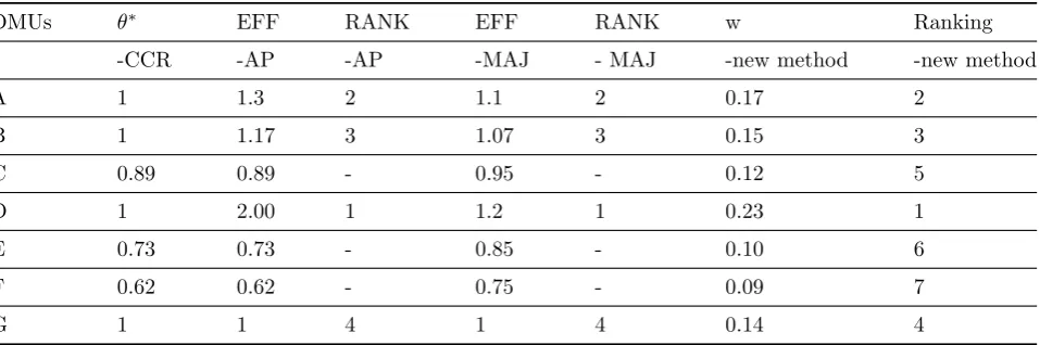
Table 4: Comparison of the results of the new method with AP and MAJ.

DMUs θ∗ EFF RANK EFF RANK w Ranking

-CCR -AP -AP -MAJ - MAJ -new method -new method

A 1 1.3 2 1.1 2 0.17 2

B 1 1.17 3 1.07 3 0.15 3

C 0.89 0.89 - 0.95 - 0.12 5

D 1 2.00 1 1.2 1 0.23 1

E 0.73 0.73 - 0.85 - 0.10 6

F 0.62 0.62 - 0.75 - 0.09 7

G 1 1 4 1 4 0.14 4

y≤ n

∑

j=1,j̸=p,q

λjyj, λj ≥0, j= 1,· · ·, n, j ̸=p, q}

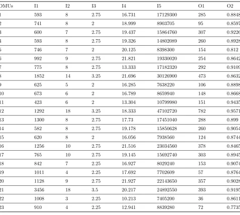
Table 5: All inputs and outputs of 23 universities.

DMUs I1 I2 I3 I4 I5 O1 O2

1 593 8 2.75 16.731 17129300 285 0.8848

2 741 8 2 18.999 8903705 95 0.8597

3 600 7 2.75 19.437 15864760 307 0.9226

4 593 8 2.75 19.326 14802089 260 0.8928

5 746 7 2 20.125 8398300 154 0.812

6 992 9 2.75 21.821 19330020 254 0.8642

7 775 8 2.75 13.333 17182320 292 0.9109

8 1852 14 3.25 21.696 30126900 473 0.8632

9 625 5 2 16.285 7638220 106 0.8898

10 673 6 2 16.789 8659940 148 0.8668

11 423 6 2 13.304 10799980 151 0.9435

12 1292 18 3.25 18.333 47102720 782 0.9571

13 1300 8 2.75 17.73 17451040 288 0.899

14 582 8 2.75 19.178 15850628 260 0.9054

15 620 8 2 16.056 7938560 124 0.8744

16 1256 10 2.75 21.516 23034560 378 0.8465

17 765 10 2.75 19.145 15692740 303 0.8945

18 842 7 2.25 16.927 8029240 153 0.9074

19 1011 4 2.25 17.692 7702609 57 0.8764

20 1128 9 2.75 21.927 22143650 357 0.9028

21 3456 18 3.5 20.217 24892550 393 0.9195

22 1008 3 2.25 10.213 7405200 36 0.8611

23 910 4 2.25 12.941 8839280 72 0.7735

E(p,Tˆp,q )=min θ

s.t:

∑n

j=1,j̸=p,qλjxj−θxp≤0

∑n

j=1,jy̸=p,qλjyj≥yp

λj ≥0, j= 1,· · ·, n, j ̸=p, q. (4.10)

In the method E(p, Tp,q) is a relative evaluation of decision making unit (xp, yp) to production possibility set (i.e. Tp,q _{). Similarly, we can define E(q, T}p,q₎ model, as follows

E(p,Tˆp,q )=min θ

s.t: ∑n

j=1,j̸=p,qλjxj−θxq ≤0

∑n

j=1,j̸=p,qλjyj ≥yq

λj ≥0, j= 1,· · ·, n, j̸=p, q. (4.11)

In fact we have evaluated DM Up andDM Uq to the production possibility set,Tp,q _{, which is obtained} from subtraction of the decision making units p and q. ,

4.2

The second stage:

Ranking by

AHP model

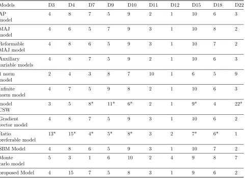
Table 6: The results of ranking the efficient DMUs by the different ranking Methods.

Models D3 D4 D7 D9 D10 D11 D12 D15 D18 D22

AP 4 8 7 5 9 2 1 10 6 3

model

MAJ 4 6 5 7 9 3 1 10 8 2

model

Reformable 4 8 6 5 9 3 1 10 7 2

MAJ model

Auxiliary 4 8 7 5 9 2 1 10 6 3

variable models

1 norm 2 4 3 8 7 10 1 6 5 9

model

Infinite 4 7 5 9 8 2 1 10 6 3

norm model

model 3 5 8* 11* 6* 2 1 9* 4 22*

CSW

Gradient 4 8 7 5 9 3 1 10 6 2

vector model

Ratio 13* 15* 4* 5* 8* 3 2 7* 6* 1

preferable model

SBM Model 4 8 6 5 9 3 1 10 7 2

Monte 5 3 1 6 10 2 4 9 8 7

carlo model

proposed Model 4 15 7 5 8 3 1 9 6 2

q.

A= [ap,q]n×n

ap,q=

E(p, Tp,q)

E(q, Tp,q₎ p, q= 1,2,· · ·, n

We take the evaluation given to unit p by the model of unitE(p, Tp,q_{) and divide it by the evaluation given} to unit q by the model of unitE(q, Tp,q_).

We have:

ap,q = 1 aq,p

, p, q = 1,2,· · ·, n

MatrixAis evaluated by DEA model in pairs, as each decision making unit attend the most optimum evalu-ation in comparison with other units. Based on pair-wise comparison matrixAby computing vectorwj, is indicator of emphasized ratio to the unitj. Therefore, we rank decision making units by these priorities.

5

Numerical example

Consider seven decision making units by two inputs for producing a normalized output in the first level as

given in Table 1. Respect to the propose method , Linear Programming model for evaluatingDM UA in set TA,B_{, is as following:}

E(A,TˆA,B )=min θ

s.t:

2λc+ 1λD+ 2λE+ 3λF+ 5λG−3θ≤0

3λc+ 5λD+ 5λE+ 4λF+ 1λG−1θ≤0

1λc+ 1λD+ 1λE+ 1λF+ 1λG≥1

λc, λD, λE, λF, λG≥0(5.12)

So Linear Programming model for evaluatingDM UB in setTA,B_{, is as following:}

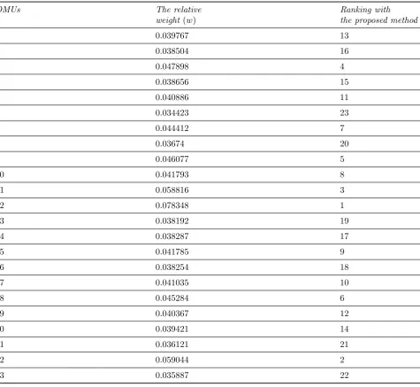
Table 7: The results of ranking by proposed Methods.

DMUs The relative Ranking with

weight (w) the proposed method

1 0.039767 13

2 0.038504 16

3 0.047898 4

4 0.038656 15

5 0.040886 11

6 0.034423 23

7 0.044412 7

8 0.03674 20

9 0.046077 5

10 0.041793 8

11 0.058816 3

12 0.078348 1

13 0.038192 19

14 0.038287 17

15 0.041785 9

16 0.038254 18

17 0.041035 10

18 0.045284 6

19 0.040367 12

20 0.039421 14

21 0.036121 21

22 0.059044 2

23 0.035887 22

s.t:

2λc+ 1λD+ 2λE+ 3λF+ 5λG−2θ≤0

3λc+ 5λD+ 5λE+ 4λF+ 1λG−2θ≤0

1λc+ 1λD+ 1λE+ 1λF+ 1λG ≥1 λc, λD, λE, λF, λG≥0(5.13)

E(A, TA,B_{) = 1.30 and E(B, T}A,B_{) = 1.44 are the} optimal answers for two Linear Programming models, then:

aA,B=

E(A, TA,B₎ E(B, TA,B₎ =

(1/44)

(1/30) = 1/11

(5.14)

aB,A=

E(B, TA,B₎ E(A, TA,B₎ =

(1/30)

(1/44)= 0/90 (5.15)

         

1 1.11 1.51 0.66 1.85 2.16 1 0.90 1 1.17 0.59 1.51 1.66 1.17 0.66 0.59 1 0.50 1.22 1.44 0.89 1.51 1.17 2 1 2 2.56 2 0.54 0.66 0.82 0.50 1 1.19 0.73 0.46 0.60 0.69 0.39 0.84 1 0.61 1 0.85 1.12 0.50 1.37 1.64 1

         

The vector w is obtained by least squares method and its results are explained in Table2. As it is seen here, efficient units are ranked in higher level than inefficient units. The proposed method presents an overall ranking for efficient decision making units.

The rank of this decision making units by the pro-posed method are explained in Table3. The rank of unitA, D, E andG has been one, because these units in relation to the other individual units are efficient in pair-wise comparison. Therefore, it is impossible to rank them in this special case, that it is one of the problems of proposed method in( 3.2). On the one hand, unit F despite has the most optimal overall pri-ority and unit B despite has the least overall pripri-ority. So in the ranking, unit F will be located in the higher level that B. The other problem of proposed method in (3.2), is that by change εs, different ranking are obtained.

In Table 4 we compare the results of the proposed model with AP andM AJ models. Efficient DMUs have same ranking in all three methods and Due to the weight vector that was resulted from paired com-parison matrix, other units have also been ranked.

6

Application

In this section, an application is used to compare these models. Finally, we analyzed the results. Consider 23 universities. each universities has five inputs: the amount of Educational environment , The number of school classes ,the number of Employee ,the number of teacher, The total budget and two outputs: the number of students, amount of Quality of education as output. All inputs and outputs are shown in Table5.

Input 2: The number of school classes. Entry 3 the number of Employee. Entry 4: the number of teacher. Entry 5: The total budget.

Output 1: The number of students. Output 2: amount of Quality of education.

These units evaluated by CCR model, DM U3,4,7,9,10,11,12,15,18,22 are efficient. Efficient DMUs are ranked. The results of ranking the efficient DMUs by the different ranking Methods are showed in Table6.

Sign (*) means DMU is inefficient. However, the weight of decision maker are used in proposed model,

the results of ranking with proposed model are shown in Table7.

As it was considered, in CSW models, some DMUs are inefficient, despite Other models were evaluated efficient then they are not ranked. DM U12 has best rank in proposed model and in most the ranking’s models. Other DMUs have same rank with all of the models. As you can see, all DMUs was ranked with the weight vector that was obtained from paired com-parison matrix. This method is the incorporation of AHP and DEA and rank all of efficient and inefficient DMUs.

7

Conclusion

We have presented a two-stage method for ranking of decision making units with incorporating DEA and AHP. In the first stage All DMUs are evaluated and compared Pairwise and in the second stage by using analytic hierarchy process, we have presented a full ranking for all DMUs. In contrast to DEA and AHP models, the advantage of the AHP/DEA approach is that it has not limitations of both DEA and AHP be-cause of using the incorporation of AHP/DEA model . The another advantage of this method is that, the pairwise comparisons matrixes of AHP are obtained mathematically from the input/output data. Thus, the evaluation is not based on subjective judgments of a decision maker. on the one hand, since we are us-ing of given inputs and outputs of DMUs, the utility theory non-axiomatic limitations of AHP are irrele-vant. The Difficulty of Sinuany-Sterns method, was that by different s, different ranking are got; but, by considering, two evaluated DMUs are removed of pro-duction possibility set in the propose model, we can not be used the proposed model for ranking the two decision making units. For future researches Future research can be study on finding a relationship be-tween obtaining weights of DEA and AHP, and using Topsis method in ranking.

References

[1] P. Anderson, N. C. Petersen, A procedure for ranking efficient units in data envelopment anal-ysis, Management Science 39 (1993) 1261-1264.

[2] R. D. Banker, A. Charnes, W. W. Cooper,Some models for estimating technical and scale ineffi-ciencies in data envelopment analysis, Manage-ment Science 30 (1984) 1078-1092.

[3] A. Charnes, W. W. Cooper, E. Rhodes, Measur-ing the efficiency of decision makMeasur-ing units, Eu-ropean Journal of Operational Research 2 (1978) 429-444.

RD projects, Management Science 37 (1991) 871-885.

[5] T. L. Saaty, The Analytic Hierarchy Process, McGrow-Hill 1980.

[6] T. L. Saaty,Decision Making the analytic hierar-chy and network processes (AHP/DEA), Journal of systems science and systems Engineering 13 (2004) 1-34.

[7] Z. Sinuany-Stern, A. Mehrez, Y. Hadad, An AHP/DEA methodology for ranking decision units, International Transactions in Operation Research 7 (2000) 109-124.

Tayebeh Rezaei Taziani, Phd stu-dent of Operations Research Faculty member of the University of Bandar Abbas- degree educator The author of 1 book-1 Research Project-2 colleague of Research Project and she has 2 Re-search Paper and 5 papers presented at national and international conferences.