DEMOGRAPHIC RESEARCH
A peer-reviewed, open-access journal of population sciences
DEMOGRAPHIC RESEARCH
VOLUME 40, ARTICLE 40, PAGES 1153–1166
PUBLISHED 7 MAY 2019
http://www.demographic-research.org/Volumes/Vol40/40/ DOI: 10.4054/DemRes.2019.40.40
Research Material
IRS county-to-county migration data,
1990–2010
Mathew Hauer
James Byars
c
2019 Mathew Hauer & James Byars.
This open-access work is published under the terms of the Creative Commons Attribution 3.0 Germany (CC BY 3.0 DE), which permits use, reproduction, and distribution in any medium, provided the original author(s) and source are given credit.
1 Introduction 1154
2 IRS migration data 1155
2.1 Comparisons to other US migration data 1157
3 Usage notes 1159
4 Data processing 1160
4.1 R code 1163
4.2 Setup 1163
4.3 Data download 1163
4.4 Data processing 1164
IRS county-to-county migration data, 1990–2010
1Mathew Hauer2
James Byars3
Abstract
BACKGROUND
The county-to-county migration data of the Internal Revenue Service’s (IRS) is an in-credible resource for understanding migration in the United States. Produced annually since 1990 in conjunction with the US Census Bureau, the IRS migration data represents 95% to 98% of the tax-filing universe and their dependents, making the IRS migration data one of the largest sources of migration data. However, any analysis using the IRS migration data must process at least seven legacy formats of this public data across more than 2000 data files – a serious burden for migration scholars.
OBJECTIVE
To produce a single, flat data file containing complete county-to-county IRS migration flow data and to make the computer code to process the migration data freely available.
METHODS
This paper uses R to process more than 2,000 IRS migration files into a single, flat data file for use in migration research.
CONTRIBUTION
To encourage and facilitate the use of this data, we provide a single, standardized, flat data file containing county-to-county one-year migration flows for the period 1990–2010 (containing 163,883 dyadic county pairs resulting in 3.2 million county-year observations totaling over 343 million migrants) and provide the full R script to download, process, and flatten the IRS migration data.
1The data and code that support the creation of this data are available online at https://osf.io/wgcf3/
?view only=c5ba62fb4821421ea0621bfd0d723e61. The data resulting from this paper is available in the Sup-plementary Materials.
2Florida State University, Tallahassee, USA. Email:[email protected].
1. Introduction
Migration flow data (i.e., the number of migrants from locationito locationj) is infor-mation that is typically difficult to obtain despite its importance (Willekens et al. 2016; Rogers, Little, and Raymer 2010). Migration scholars typically focus on cross-border, international migration flow data, and recent country-to-country migration data is vital for understanding migration processes (Abel and Sander 2014; Abel 2017, 2013). How-ever, there is growing demonstrated importance surrounding subnational migration flows (Sorichetta et al. 2016; Curtis, Fussell, and DeWaard 2015).
In the United States, subnational migration flow data is available from three primary sources, depending on the time period: the Decennial Census, the American Community Survey, and the IRS’s county-to-county migration data (described in detail in the corre-sponding section below). The IRS migration data is a pioneering use of administrative records to estimate demographic processes and is available on an annual basis since 1990. Because of the annual availability, relatively large, long time series universe due to the ad-ministrative records, and long history of use, the IRS data is an attractive data source for conducting migration research in the United States (e.g., Curtis, Fussell, and DeWaard 2015; Molloy, Smith, and Wozniak 2011; Frey 2009). Unfortunately, this data exists in seven legacy formats, split between 2,000+ data files, making analysis with this data rather burdensome and has probably hindered the widespread adoption of this valuable resource for US migration scholarship.
To encourage and facilitate the use of this tremendous migration resource, we make two contributions: (1) We publish a single, flat, standardized data file containing all county-to-county one-year migration flows for the period 1990–2010 (containing 163,883 dyadic county pairs resulting in 3.2 million county-year observations, totaling over 343 million migrants). (2) For reproducibility, transparency, and educational purposes, we publish the open-source R code used to process the IRS data into the single, flat, stan-dardized data file. Scholars who wish to use this data should still familiarize themselves with the strengths and weaknesses, idiosyncrasies, and design of this data (see Gross 2005; Engels and Healy 1981; Franklin and Plane 2006; Pierce 2015 for discussions on the IRS data) and with the procedures outlined in this document and in the corresponding R code.3
We have attempted to introduce as little postprocessing as possible to process the data into a common format. US counties are fairly stable geographic units, but some changes in county boundaries, names, and Federal Information Processing Standard Pub-lication (FIPS) codes do occasionally occur.4To try and keep as close to the original data fidelity as possible, we did not recode any geographic changes and present the IRS
migra-3 The R code used to produce this data is available in an online repository located at https://osf.io/
wgcf3/?view only=c5ba62fb4821421ea0621bfd0d723e61.
tion data as-is. For instance, Broomfield County, Colorado (FIPS 08014), was created out of parts of Adams, Boulder, Jefferson, and Weld counties in 2001, and thus has data only after 2002. Users should be aware of any changes in county boundaries, county names, or FIPS changes that could substantially alter any analysis of this data.5
We organize the document as follows: First, we describe the IRS county-to-county migration data to provide an overview of the data for scholars who might be unfamiliar with the IRS migration data. Second, we provide usage notes that supply important infor-mation that may assist other researchers who want to use our data. Third, we describe our single, flat, standardized file and document important nuances in the raw IRS migration data. Finally, we describe parts of the R code used to download the IRS migration data and process it into a common format.
The IRS migration data is an incredible tool for understanding migration. By pro-viding this data in a readily available format and the subsequent open-source computer code used to process this data, we hope to facilitate its use in descriptive, exploratory, and analytic research of migration in the United States. This data is particularly useful for un-derstanding migration as a spatial entity and for investigating the evolution of migration systems over time.
2. IRS migration data
The IRS began using tax data to estimate migration in the 1970s and 1980s (Engels and Healy 1981; Franklin and Plane 2006) and began releasing migration data in 1990. The IRS uses individual federal tax returns, matches these individual returns between two tax years (for instance tax year 2000 and tax year 2001), and identifies migrants and nonmigrants. Beginning with tax year 1991 (migration year 1990), the IRS produces this data in conjunction with the US Census Bureau using the IRS Individual Master File, which contains every Form 1040, 1040A, and 1040EZ (Gross 2005). Migration is identified when a current year’s tax form contains an address that is different from the matched preceding year’s return. A nonmigrant is identified when there is no change in address between two years. For the 2002 tax year, the IRS migration data contained approximately 130 million returns (Gross 2005).
The annual series of county-to-county migration data covers 95% to 98% of the tax-filing universe (or approximately 87% of US households (Molloy, Smith, and Wozniak 2011)) and their dependents, making this data the largest migration data source for count
5 More detailed information about county boundary, name, or FIPS changes can be
found at the following locations: https://www.census.gov/geo/reference/county-changes.html,
flows between counties in the United States. The IRS derives migration information from tax filings, making those who do not file taxes most likely to be underrepresented in the migration data (Gross 2005; DeWaard, Curtis, and Fussell 2016), namely undocu-mented populations, the poor, the elderly, and college students (Gross 2005). However, the overwhelming majority of householders file US tax returns in the United States (Mol-loy, Smith, and Wozniak 2011).
The IRS reports a number of important variables in their data. They identify the origin and destination counties, the number of tax returns or filers associated with those moves (roughly analogous to the number of households and listed as thereturnsfield in the raw data) who moved from countyito countyj, and the number of tax exemptions associated with those moves (roughly analogous to the number of individuals and listed as
theexemptionsfield in the raw data). They also report the number of nonmigrants,
re-ported as the number of tax returns and exemptions associated with migrants from county ito countyi. We treat theexemptionsfield as the total number of migrants.
Between 1990 and 2010, the IRS used the same procedures to process the county-to-county migration data. However, in 2011 the IRS introduced a new method for processing the migration data and introduced ‘enhancements’ to improve the overall quality of the data (Pierce 2015). The IRS introduced three major changes. First, they began basing mi-gration on a full year of data as opposed to a partial year of data. To meet Census Bureau deadlines, the IRS processed all income tax returns filed before the end of September and did not process the returns filed between the end of September and the end of the calendar year. Beginning with migration year 2011, the IRS included the approximately 4% of returns that are filed between the end of September and December 31, allowing the IRS to produce a full calendar year’s worth of migration. Second, the IRS improved the year-to-year matching, increasing the number of matched returns by 5%. Prior to 2011, the IRS used only the primary filer’s taxpayer identification number (TIN), potentially excluding individuals who may be listed as a dependent in year 1 but file on their own in year 2, or in cases where a secondary filer in year 1 (such as a spouse) files as a primary filer in year 2. After 2011, the IRS broadened their matching process to include primary, secondary, and dependent TINs to improve the matching process by 5%. Third, the IRS began tabulating gross migration at the US state level by size of adjusted gross income (AGI) and the age of the primary taxpayer.
2.1 Comparisons to other US migration data
As stated in the preceding section, the three main sources of migration data in the United States are the Decennial Census long form, the American Community Survey, and the IRS county-to-county migration data.
Up to and including Census 2000, the long form of the Decennial Census contained the question “Where did you live five years ago?” This question provided five-year migra-tion data once every decade. With the discontinuamigra-tion of the long form in Census 2010, the Census Bureau began collecting migration information on the American Community Survey (ACS) with the question “Where did you live one year ago?” This question pro-vides one-year migration data with each ACS release.
The Decennial long form was a robust sample, surveying approximately one in every six (16.7%) US households. The ACS is a smaller survey with a sample size of approxi-mately 2 million US households per year. Due to the smaller sample size, the Census Bu-reau pools responses into five-year averages for county-to-county migration data. Thus, ACS migration data represents one-year migration data over a five-year period. The Cen-sus Bureau processes the ACS migration data and releases county-to-county migration data sets on an annual basis, reflecting the five-year average (2010–2014, 2011–2015, etc.).
The ACS migration products and the IRS migration data both have strengths and weaknesses. Table 1 compares the ACS migration products with the IRS migration data in some key areas. The ACS universe is more complete than the IRS migration universe, lacking the tax-paying universe bias present in the IRS data; however, the ACS migration data contains approximately 2% of the observations in the IRS migration data. The IRS releases the migration data annually, allowing annual comparisons while the Census Bu-reau suggests only nonoverlapping five-year products should be compared to each other (i.e., 2005–2009 and 2010–2014) (Brown 2009).
Table 1: Comparison between American Community Survey and IRS county-to-county migration data
Issue ACS Migration Products IRS Migration Data
Sample size Approximately 2 million households per year 116 million+ households Data universe Sample is all US households Universe is tax-filing households Coverage period 2005–2016 1990–2016
Time period reported Five-year average Annual
Demographic Each five-year product reports different No demographic characteristics characteristics sociodemographic characteristics (e.g., 2010–2014
contains relationship, household type, and tenure, 2011–2015 contains age/sex/race/Hispanic origin
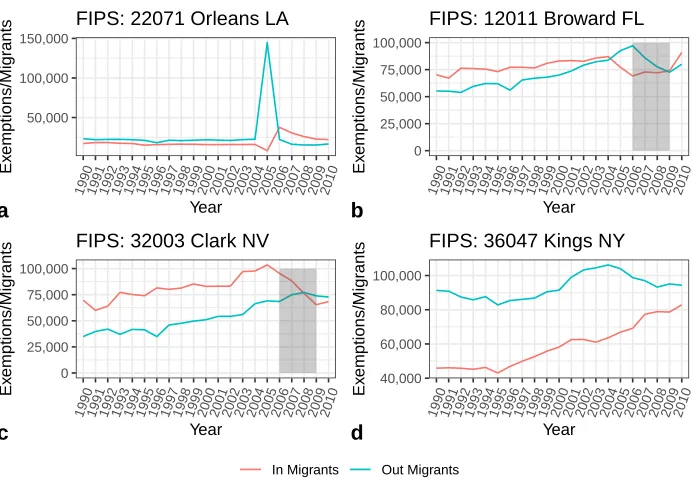
changes in migration flows aggregated to gross-migration flows in four sample counties. These four sample counties are just some of the easily detectable impacts of major US events such as Hurricane Katrina in 2005 (Curtis, Fussell, and DeWaard 2015) or the Great Recession. These migration changes are largely undetectable in the ACS migration data or our ability to detect such changes is hampered by the five-year release.
Figure 1: Sample migration streams from the IRS migration data
50,000 100,000 150,000
1990 1991 1992 1993 1994 1995 1996 1997 1998 1999 2000 2001 2002 2003 2004 2005 2006 2007 2008 2009 2010
Year
Ex
emptions/Migr
ants
FIPS: 22071 Orleans LA
a 0 25,000 50,000 75,000 100,000
1990 1991 1992 1993 1994 1995 1996 1997 1998 1999 2000 2001 2002 2003 2004 2005 2006 2007 2008 2009 2010
Year
Ex
emptions/Migr
ants
FIPS: 12011 Broward FL
b 0 25,000 50,000 75,000 100,000
1990 1991 1992 1993 1994 1995 1996 1997 1998 1999 2000 2001 2002 2003 2004 2005 2006 2007 2008 2009 2010
Year
Ex
emptions/Migr
ants
FIPS: 32003 Clark NV
c
40,000 60,000 80,000 100,000
1990 1991 1992 1993 1994 1995 1996 1997 1998 1999 2000 2001 2002 2003 2004 2005 2006 2007 2008 2009 2010
Year
Ex
emptions/Migr
ants
FIPS: 36047 Kings NY
d
In Migrants Out Migrants
Note: The annual release of the IRS migration data allows for detection of rapid changes in migration streams. The effect of Hurricane Katrina on New Orleans, LA, (a) is clearly visible by the large increase in out-migration in 2005. The moderate effect of the US housing bubble burst and Great Recession is detectable in Broward, FL, (b) and a much greater effect in Clark, NV, (c) as evidenced by the decline in in-migration during the 2006–2009 period. Even migration streams nearly unaffected by major US changes are also detectable, as is the case in Kings, NY, (d) which appears only marginally affected by the Great Recession or the 9/11 tragedy in 2001. These migration changes are largely undetectable in the ACS migration data or our ability to detect such changes is hampered by the five-year release. These are just a few examples of what is possible with the IRS migration data.
more appropriate. If a migration scholar were interested in the sociodemographic details of migration, the ACS migration products would be more appropriate.
Despite these limitations, scholars have successfully used the IRS migration data to forecast interstate migration (Isserman et al. 1985), investigate migrant destinations after Hurricane Katrina (Curtis, Fussell, and DeWaard 2015), other broader spatial patterns of migration (Henrie and Plane 2008), and to examine possible explanations (Molloy, Smith, and Wozniak 2017) to the Great Recession’s migration slowdown (Frey 2009). Making this data more easily available in a more standardized format to a broader set of migration scholars can further our understanding of migration above and beyond the ACS data.
3. Usage notes
The dataset generated here provides detailed county-to-county one-year migration data based on administrative records. Users of this data should be aware that although the data has been prepared in a transparent manner with documentation of its creation and postprocessing, and with open-source computer code, little was done to postprocess the data to correct any possible inconsistencies or errors. This data should be used only with full awareness of the inherent limitations of the IRS migration data and with the knowledge of the procedures outlined in this document and in the corresponding R code. Caveat emptor – users beware.
Users should be aware of several limitations of the IRS data. Namely, that any origin-destination pair with fewer than ten tax filers is censored or suppressed by the IRS for privacy reasons. We have collected these censored flows into a unique FIPS code (FIPS 99999) by subtracting all uncensored flows from the total number of migrants. Any origin-destination pair with fewer than ten tax filers over the entire period is thus excluded from the final data file since no data would be recorded in the IRS data file due to censoring.
Users should also be mindful of possible geographic changes to county boundaries that could affect the data.
The county migration data we present comes from theexemptionsfield of the IRS migration data. The original IRS migration data contains two consistent fields across all years of data: areturnsfield and anexemptionsfield. Returns are the number of tax returns filed, while exemptions are a proxy for the members of the household. We use the number of exemptions to better mimic the number of individuals migrating rather than the number of households.
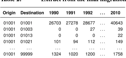
Table 2: Extract from the final migration data file
Origin Destination 1990 1991 1992 . . . 2010
01001 01001 26703 27278 28677 . . . 40643 01001 01003 0 0 27 . . . 39 01001 01013 0 0 0 . . . 22 01001 01021 101 94 112 . . . 149 . . . . 01001 99999 1324 1020 1200 . . . 1758
Note: Origins and Destinations are the five-digit FIPS codes, with 99999 representing all destinations with flows fewer than ten filers. The counts represent the number ofexemptionsin the IRS data. Nonmigrants are identified as having the same FIPS codes in the Origin and Destination fields.
4. Data processing
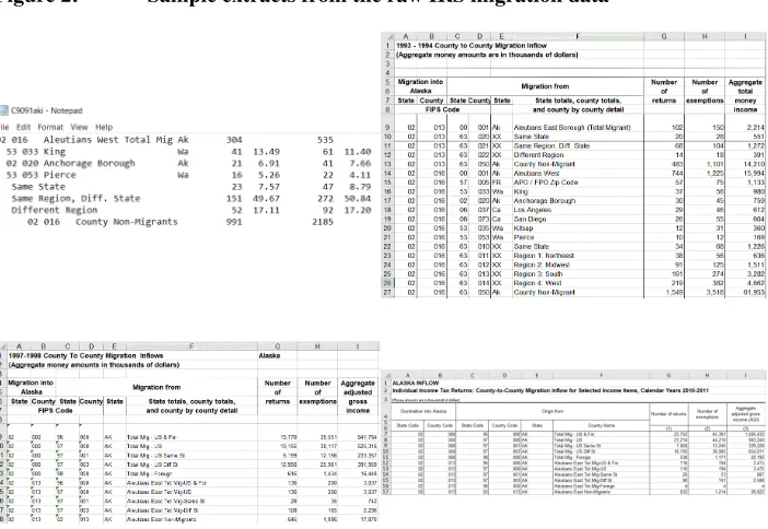
Figure 2: Sample extracts from the raw IRS migration data
Note: Here are four sample raw data extracts for 1990, 1993, 1997, and 2010. Note that all four have different file formats, structures, and coding schemes.
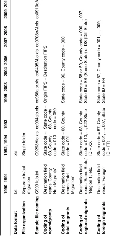
Table 3: Select differences in the file formats, file organizations, naming, and treatment of various migration statistics
1990–1991 1992, 1994 1993 1995–2003 2004–2006 2007–2008 2009–2010 Data format txt xls File or ganization Separ ate in/out Single folder mig ration Sample file naming C9091alo .txt C9293Alo .xls co934alo .xls co956alor .xls co0405ALo .xls co0708oAl.xls co0910oAL.xls Coding of Destination field State code = State code = Or igin FIPS = Destination FIPS nonmigrants reads ’County 63, County 63, County Non-Mig rants’ code = 010 code = 050 Coding of Destination field State code = 00, County State code = 96, County code = 000 total migrants reads ’T otal code = 001 Mig ration’ Coding of Destination field State code = 63, County State code = 58 or 59, County code = 000, ..., 007, regional migrants reads ’Same State ,’ code = 010, ..., 022 State State ID = SS (Same State) or DS (Diff State) ’Region 1, ’ etc. ID = XX Coding of Destination field State code = 57, County State code = 57, County code = 001, ..., 009, foreign migrants reads ’F oreign’ code = 001, ..., 007, State State ID = FR ID = FR
number of enumerated migrants (the migration flows with greater than ten migrants) from the total number of migrants. This way, the sum of all enumerated migrants in our dataset equals the total number of migrants in the IRS dataset. And the sum of all migrants and nonmigrants for any origin in a given year should roughly approximate the county population estimate for the previous year.
The aggregation to FIPS 99999 is the only mathematical postprocessing of the IRS data.
4.1 R code
The R code used to produce this data is available in an online repository.6The code makes use of multicore processing to speed up computation time. There are three main sections in the code: a setup section, a data download section, and a data processing section. The final flat file,county migration data.txt, contains the # of exemptions and can be either downloaded at GitHub or produced by running the R code.
4.2 Setup
The script000-libraries.Rsimply sets up the R workspace to facilitate the data processing. The appropriate R packages are downloaded and installed if the user does not already have these packages installed. The parallel computing environment is also set up asDetectCores() - 1to ensure that the computer has appropriate resources for other tasks. The script requires a single reference tab-separated (tsv) file in this section, and we load it into the local environment. Theref state.tsvfile contains FIPS code information for US states. We simply add a FIPS state code for ‘unknown’ and assign it FIPS state 99.
4.3 Data download
The script001-download data.Rdownloads and unzips the migration data from the IRS’s websites and saves the formatted data in a standard file folder in the subdirectory
MigData/.The IRS data is in two primary formats: 1990–2003 and 2004-onward. The
IRS includes eight files in their zip archives that contain no data (these are in years 1998, 1999, 2000, and 2001). We delete these files after downloading and unzipping them. If they are not deleted, they cause the subsequentfor loopsto fail in the next section. These files do not contain any migration information, and their names suggest they rep-resent aggregation of migration flows (for example ‘co990usi.xls’ suggests county (co)
years 1999–2000 (990) for US (us) in-migration (i)), and we are unsure exactly why the IRS included these files or their purpose.
4.4 Data processing
References
Abel, G.J. (2013). Estimating global migration flow tables using place of birth data.
Demographic Research28(18): 505–546.doi:10.4054/DemRes.2013.28.18.
Abel, G.J. (2017). Estimates of global bilateral migration flows by gender between 1960 and 2015.International Migration Review(online). doi:10.1111/imre.12327.
Abel, G.J. and Sander, N. (2014). Quantifying global international migration flows. Sci-ence343(6178): 1520–1522. doi:10.1126/science.1248676.
Brown, W.A. (2009). A compass for understanding and using American Community Survey data: What researchers need to know. Suitland: US Census Bureau.
Curtis, K.J., Fussell, E., and DeWaard, J. (2015). Recovery migration after Hurricanes Katrina and Rita: Spatial concentration and intensification in the migration system.
Demography52(4): 1269–1293. doi:10.1007/s13524-015-0400-7.
DeWaard, J., Curtis, K.J., and Fussell, E. (2016). Population recovery in New Orleans after Hurricane Katrina: Exploring the potential role of stage migration in migration systems.Population and Environment37(4): 449–463. doi:10.1007/s11111-015-0250-7.
Engels, R.A. and Healy, M.K. (1981). Measuring interstate migration flows: An origin– destination network based on internal revenue service records.Environment and
Plan-ning A: Economy and Space13(11): 1345–1360.
Franklin, R.S. and Plane, D.A. (2006). Pandora’s box: The potential and peril of mi-gration data from the American Community Survey. International Regional Science
Review29(3): 231–246. doi:10.1177/0160017606289895.
Frey, W. (2009). The great american migration slowdown. Washington, D.C.: Brookings Institution.
Gross, E. (2005). Internal Revenue Service area-to-area migration data: Strengths, limi-tations, and current trends. Washington, D.C.: Internal Revenue Service (SOI Working Paper).
Henrie, C.J. and Plane, D.A. (2008). Exodus from the California core: Using demo-graphic effectiveness and migration impact measures to examine population redistribu-tion within the western United States. Population Research and Policy Review27(1): 43–64.doi:10.1007/s11113-007-9053-6.
Isserman, A.M., Plane, D.A., Rogerson, P.A., and Beaumont, P.M. (1985). Forecasting interstate migration with limited data: A demographic-economic approach.Journal of
Molloy, R., Smith, C.L., and Wozniak, A. (2011). Internal migration in the United States.
Journal of Economic Perspectives25(3): 173–196.doi:10.1257/jep.25.3.173.
Molloy, R., Smith, C.L., and Wozniak, A. (2017). Job changing and the decline in long-distance migration in the United States. Demography54(2): 631–653. doi:10.1007/ s13524-017-0551-9.
Pierce, K. (2015). SOI migration data: A new approach: Methodological improvements for SOI’s United States population migration data, calendar years 2011–2012. Wash-ington, D.C.: Statistics of Income, Internal Revenue Service.
Rogers, A., Little, J., and Raymer, J. (2010).The indirect estimation of migration:
Meth-ods for dealing with irregular, inadequate, and missing data. Dordrecht: Springer.
Sorichetta, A., Bird, T.J., Ruktanonchai, N.W., zu Erbach-Schoenberg, E., Pezzulo, C., Tejedor, N., Waldock, I.C., Sadler, J.D., Garcia, A.J., Sedda, L., and Tatem, A.J. (2016). Mapping internal connectivity through human migration in Malaria endemic countries.Scientific Data3(160066): 1–16.doi:10.1038/sdata.2016.66.