Reinforcement Learning Agent under Partial Observability for Traffic Light Control in Presence of Gridlocks

for Traffic Light Control in Presence of Gridlocks

Thanapapas Horsuwan

_{and Chaodit Aswakul}

International School of Engineering, Faculty of Engineering, Chulalongkorn University

[email protected]

2 _{Wireless Network and Future Internet Research Unit,}

Department of Electrical Engineering, Faculty of Engineering, Chulalongkorn University

[email protected]

Abstract

Bangkok is notorious for its chronic traffic congestion due to the rapid urbanization and the haphazard city plan. The Sathorn Road network area stands to be one of the most critical areas where gridlocks are a normal occurrence during rush hours. This stems from the high volume of demand imposed by the dense geographical placement of 3 big educational institutions and the insufficient link capacity with strict routes. Current solu-tions place heavy reliance on human traffic control expertises to prevent and disentangle gridlocks by consecutively releasing each queue length spillback through inter-junction coordination. A calibrated dataset of the Sathorn Road network area in a microscopic road traffic simulation package SUMO (Simulation of Urban MObility) is provided in the work of Chula-Sathorn SUMO Simulator (Chula-SSS). In this paper, we aim to utilize the Chula-SSS dataset with extended vehicle flows and gridlocks in order to further optimize the present traffic signal control policies with reinforcement learning approaches by an artificial agent. Reinforcement learning has been successful in a variety of domains over the past few years. While a number of researches exist on using reinforcement learning with adaptive traffic light control, existing studies often lack pragmatic considerations con-cerning application to the physical world especially for the traffic system infrastructure in developing countries, which suffer from constraints imposed from economic factors. The resultant limitation of the agent’s partial observability of the whole network state at any specific time is imperative and cannot be overlooked. With such partial observability con-straints, this paper has reported an investigation on applying the Ape-X Deep Q-Network agent at the critical junction in the morning rush hours from 6 AM to 9 AM with practi-cally occasional presence of gridlocks. The obtainable results have shown a potential value of the agent’s ability to learn despite physical limitations in the traffic light control at the considered intersection within the Sathorn gridlock area. This suggests a possibility of further investigations on agent applicability in trying to mitigate complex interconnected gridlocks in the future.

1

Introduction

project Sustainable Mobility Project 2.0 of the World Business Council for Sustainable Develop-ment (WBCSD), the Sathorn Model Project was adopted by the Toyota Mobility Foundation in Bangkok [21]. Various sensors have been installed along the upstream lanes approaching the critical Surasak Intersection by the project [21]. In early attempts to mimic real world congestions for what-if scenario studies, the work of Chula-Sathorn SUMO Simulator (Chula-SSS) [3] has been initiated to provide calibrated datasets over the Sathorn Road network in a microscopic road traffic simulation package Simulation of Urban MObility (SUMO) [15]. The datasets has been extensively calibrated by the root mean squared error (RMSE) of the actual link travel time in the weekday morning and evening rush hour from 6 AM to 9 AM and 3 PM to 7 PM respectively.

One of the what-if scenarios of utmost importance is to investigate on different congestion mitigation plans especially on traffic signal light controls. In doing so, there exist numerous challenges. The Sathorn Road infrastructure stands to be the busiest road network [24]. This is due to the density of the high rise buildings and the dense geographical placement of the schools and universities. No automation has been trusted for rush-hour traffic signal light control op-erations, although such automation infrastructure has already been installed. Currently, in practice, a manual adaptive traffic signal control is utilized, which relies on tacit knowledge ac-cumulated by traffic police expertise. The current traffic indicators gained through the expert’s experience are the queue length and vehicle minimum gap. Although heuristic signal actuated logics were extracted from human experts as an attempt to standardize the process [3], human expertise is still heavily relied on and current tools are utilized for visualization, simulation, and further analysis. In overall, hence, the traffic signal light control problem remains an open challenge to explore further towards an optimization and automation within the present traffic signal control policies. In addition, due to severely over-saturated condition, gridlocks are a normal occurence in the time of rush hour. This requires the traffic police’s manual intervention and coordination to resolve in current practices, and complicates further if such operation must be automated in the future.

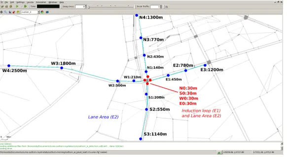
(a) Longdo Map (with granted usage permission

fromhttp://map.longdo.com/ (b) Chula-SSS Dataset in SUMO

Figure 1: Comparison between actual map and Chula-SSS dataset in the Sathorn Road Area

definitions are mostly hard to observe by a real agent, such as delay [2, 6, 28, 19] or vehicle waiting time [8,28]. There remain many open challenges consequently.

Especially for the traffic system infrastructure in developing countries, this paper tries to investigate one challenge, stemming from constraints imposed from economic factors. Partic-ularly, this paper addresses the resultant limitation of the agent’s partial observability of the whole network state at any specific time, which is imperative and cannot be overlooked. With such partial observability constraints, this paper has reported an investigation on applying the Ape-X Deep Q-Network agent at the critical junction in the morning rush hours from 6 AM to 9 AM with practically occasional presence of gridlocks. The obtainable numerical exper-iments utilize heavily Chula-SSS dataset with the focus on studying a potential value of the agent’s ability to learn despite physical limitations in the traffic light control at the considered intersection within the Sathorn gridlock area.

The paper is organized as follows: Section 2 describes the problem and defines the agent; the experimental setup is in Section 3 and discussion of the results in Section 4; finally, we conclude the paper in Section5.

2

Problem Formulation

In this section, we first introduce the existing traffic infrastructure, the corresponding simulation model, and then formulate the traffic light control problem as an reinforcement learning task.

2.1

Sathorn Road Infrastructure

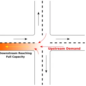
Figure 2: Example scenario for Gridlock

and to ease the manual callibration process. The vehicle flows of the dataset are callibrated only on predefined routes occuring on the major roads.

Traffic Gridlock: A traffic gridlock is a form of congestion state where queue length spillback propagates in a closed loop–resulting in a complete standstill. Once the downstream edge approaches full capacity, the limited capacity would disallow the upstream edges to enter upon a green light phase. In practice, this would lead to vehicles being trapped in the middle of the junction, blockading the path for the opposite direction–rendering any phase changes ineffective. These gridlocks are frequently observed in the Sathorn Road network at the time of peak traffic demand, requiring traffic experts to manually disentangle the gridlock through inter-junction coordination.

The Chula-SSS SUMO dataset was calibrated under SUMO v0.25.0 when the vehicle lane changing model was not properly configured, leading to criss-cross lane-to-lane connections. The vehicle behavior inside these intersecting internal links is not supported in the current SUMO v1.0.1 version. The dataset is adviced to run with the flag --no-internal-links true, disallowing vehicle junction blockers altogether. Although the Chula-SSS SUMO dataset was not calibrated for vehicle junction blockade, gridlocks through queue length spillback still occur for upstream demand when the downstream edge is at full capacity. In the case that the downstream capacity is full, SUMO’sno-block-heuristic mechanism will not allow the vehicles in the upstream to move into the junction. An example scenario for gridlock can be illustrated by Figure2, where the upstream demand from the North, West, and South directions all try to utilize the East downstream lane. If the lane capacity is not enough or there is not enough flow, the lane then becomes a traffic bottleneck and queue length spillback will occur and the vehicles in the upstream demand will be unable to flow.

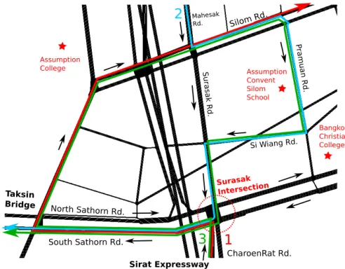
Figure 3: Critical Routes in the Sathorn Network

Table 1: Extended Route Flows

Route Time Flow (Vehicles per hour) Total Vehicles

1 7:00 AM - 8:15 AM 425 531

2 6:45 AM - 7:15 AM 300 150

3 6:15 AM - 6:45 AM 300 150

proceeding to the Silom Road. Routes 2 and 3, color-coded by blue and green respectively, represents parents living in the West side–seen by the need to cross the Chao Phraya River by the Taksin Bridge. The difference between the two routes is the origin, Route 2 comes from the North Mahesak Road while Route 3 comes from the South Sirat Expressway. The flows in each route are estimated by statistical surveys at each educational institution regarding the total number of students that come by private cars as shown in Table1. It can be observed that the 3 critical routes all utilize the downstream South Sathorn Road. It can be expected that the downstream South Sathorn Road will most likely be the bottleneck link that could potentially cause gridlock once it approaches full capacity.

The Surasak Intersection is the main junction of interest. The current traffic fixed-time control signal phase handcrafted by human experts is defined in Figure4. The main phases as defined by the traffic police experts are phase 1, 3, and 5. However, based on the extracted heuristic signal actuated logics from human experts [3] as shown in Figure4, extra phases which are the subset of other phases like phase 4 and 6 are also utilized in special cases to mitigate gridlock.

Standard Phase 1-3-1-5 Changing Phase from 1 to 3:

• When the queue of downstream North Sathorn reaches the Sathorn Intersection

• When the queue of downstream South Sathorn reaches the Sathorn Intersection

• Queue of Si Wiang Road reaches Pramuan Road on Bangkok Christian College and Assumption Convent School

• Vehicles on Taksin Bridge 300 meters from Sathorn Intersection is starting to move

• Phase 1 duration more than 120-150 seconds

Changing Phase from 3 to 1:

• Reduced jam length of Si Wiang Road or vehicles are moving on Pramuan Road continuously for 20-30 seconds

• Minimum gap between vehicles that crosses the intersection is too high

• Velocity of the vehicles that crosses the intersection is too low

• Phase 3 duration more than 30-80 seconds

Changing Phase from 1 to 5:

• Queue of Si Wiang Road reaches Pramuan Road on Bangkok Christian College and Assumption Convent School

• Queue of CharoenRat is too long

• Phase 1 duration more than 120-150 seconds

Changing Phase from 5 to 1:

• Reduced jam length of CharoenRat Road

• Phase 5 duration more than 40-50 seconds

Note: Use Phase 1-3-1-3-5 if want to get cars out from Surasak and Pramuan Road. Use Phase 4 (instead of Phase 1) when the head of queue from Sathorn South reaches Sathorn Intersection. Use Phase 6 (instead of Phase 1) when the head of queue from Sathorn North reaches Sathorn Intersection.

Figure 5: Sensor Configuration with granted usage permission fromhttp://map.longdo.com/

Figure 6: Detector Configuration in SUMO

their presence is necessary for the learning ability. And we rely on the simulation capability of SUMO together with our chosen learning algorithm to help convey this justification for future engineering investment, if a learning-based traffic light control framework would be envisioned for a possible future deployment.

2.2

Reinforcement Learning

To formulate a traffic light control as a reinforcement learning problem, we consider tasks in which an agent interacts with the envionmentE, in this case the SUMO simulation, in a sequence of observations, actions, and rewards. At each time steptthe agent receives a representation of the environment’s statest, the agent responds by selecting an actionat, and the environment

executes the action and returns back the next rewardrt+1and statest+1. The goal of the agent is a policyπwhich maximizes the expected cumulative discounted rewardRt=P

inf

k=0γ

k_r t+k+1.

State Space

LetSe

t be the environment internal state at time steptandStabe the agent’s internal

represen-tation of the state at time stept. The environment’s internal stateSe

t is not directly observed by

the agent; instead the agent observes sensory information output from the simulated detectors. The simulated detectors are placed in correspondance with the actual geographical placement of the sensors as explained in Section2.1. Therefore, the only available observationOfor the agent will be the occupancy values from each sensor and the current traffic signal phaseP. The traffic signal phaseP is a one-hot encoding of the traffic phase index, each element represents a different traffic phase, henceP is a binary vector with the size of action spaceA, P ∈B|A|. There are a total of 21 cells in the system (18 upstream cells and 3 downstream cells). The agent’s state space will then be the vectorSa _∈

R21×P. In SUMO, the mean occupancy for each lane area detector is defined as the mean percentage of the occupied detector’s place by vehicles. However, a cell may span several edges, consisting of lane area detectors of unequal length. To find the mean occupancy, the weighted average of the mean occupancy with respect to the detector length is used.

Note that the agent has partial observabilityOt=Sta6=Ste, and the agent’s limited visibility

does not contain enough information for the states of the other critical intersections in the grid. Although this is a partially observable Markov decision process (POMDP), we will investigate the effectiveness of the observation under the assumption that the current observation is the environment state to limit the complexity of the architecture. While it is also possible to build

Sa

t through the complete historySta =Ht, the beliefs of the environment stateSta = (P[Ste =

s1], ...,P[Ste=s

n_{]) [13], or using a recurrent neural network S}a t =σ(S

a

t−1Ws+OtW0) [29], we will leave that up for future works to extend.

Action Space

After the agent receives a representation of the environment’s statesa

t ∈ S at the beginning of

time stept, the agent is required to select an actionat∈ A to influence the system dynamics.

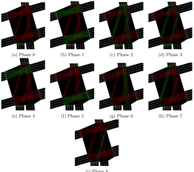
(a) Phase 0 (b) Phase 1 (c) Phase 2 (d) Phase 3

(e) Phase 4 (f) Phase 5 (g) Phase 6 (h) Phase 7

(i) Phase 8

Figure 7: Action Space Consisting of 9 Phases

previous action at−1, then a transition of traffic signal is executed before the selected action

at. The transition signal is defined as 5 seconds of yellow light for lanes that have previously

received green light.

Reward

The immediate feedback signal after the agent takes an actionatis the scalar rewardrt+1∈R. With the limited visibility of the agent, the rewardrt+1in this research is shown in Equation (1): the weighted difference between the vehicle throughput during time stept tot+ 1 denoted by

µt+1 and weighted observed occupancy. The vehicle throughput is provided by the induction loop detectors, and the weighted observed occupancy is from the observation in the next time step Ot+1. Note that the use of the subscript t+ 1 in the reward is intentional as to place emphasis on the chronological flow of receiving delayed reward the time step after taking an actionat, by which the agent is able to observe the new statest+1.

whereby α ∈ _R+ _{and β ∈}

R+ are non-negative constants to vary the ratio between the two terms. As defined in the agent’s state, the observation vector O ∈ _R21_{×P comprises of 18} occupancy values for each upstream cell, 3 occupancy values for each downstream cell, and the one-hot encoding of the traffic signal phase. To limit the agent’s punishment for vehicles that are too far away, only the first 3 cells in each upstream approaching cells are taken into account. The occupancy values from the observation vector will then be dot product by the maximum cell capacityC, which is a vector containing the maximum cell capacity for the first 3 upstream approaching cells. The maximum cell capacity is defined as the maximum number of vehicles that is able to fit inside a cell without minimum gap length. The resulting product would give the total vehicle backlog of all of the approaching lanes with respect to the 3 approaching cells. In this paper, we will investigate the effects of varying the parametersαandβin the reward function.

Agent Architecture

We model the learning agent to learn in a distributed setting with Ape-X [11]. The Ape-X architecture is a general learning framework which centralizes a shared replay memory and uses prioritized experience replay [20] to learn the most useful experiences. Different exploration policies can be given to the different distributed actors. This framework may be combined with different learning algorithms, where we have combined it with Deep Q network (DQN) [16,17] without the convolutional layers due to the low spatial dimensionality of the input. With the numerous improvements and proposed extensions to the architecture [25,26,20,4,7], we have chosen to utilize some of the extensions of Rainbow [10] as proposed in Ape-X DQN.

Vanilla DQN: A deep Q network (DQN) is a multi-layered neural network that estimates the action-value functionQ(s, a;θ)≈Q∗(s, a), withθas the parameters. Two important com-ponents of the DQN are the experience replay and the target slowly moving copy of the online network with parameters θ− [17]. The experience replay [12] stores the agent’s experiences

et= (st, at, rt, st+1) and batches are sampled from the pool uniformly ie. (s, a, r, s0)∼U(D). The notation without t is to denote that the sampled experience need not be at the current timet, but any experience from the replay buffer. The Q network can be trained by adjusting the parameters θt to reduce the mean-squared error in the Bellman equation. The following

loss function at training steptis the squared Temporal Difference (TD) error.

Lt(θt) =

1

2E(s,a,r,s0)∼U(D)

r+γmax

a0 Q(s 0_{, a}0_;θ−

t)−Q(s, a;θt 2

Ape-X DQN: The extensions that we have chosen from Rainbow [10] includes: Double Q-Learning [25] to lower the overestimation bias due to the use of the max operator, Prioritized Replay [20] to increase data efficiency of the samples by importance weighted with absolute TD error, Dueling Networks [26] to improve the generalization of the agent by learning the value of each state, and Multi-step learning [22] for faster convergence.

Ape-X DQN [11] combines the aforementioned improvements in a single integrated agent. A dueling network architecture is used as the function approximatorQ(·,·, θ). The loss function is then:

Lt(θt) =

1

2E(s,a,r,s0)∼pt(D)

"

r(n)+γnQ(s(n),argmax

a

The experiments have been conducted by using RISELab’s RLlib [14], an open-source library for reinforcement learning that uses Ray [18] for distributed execution and Tensorflow [1] for model definition. We have built an OpenAI Gym [5] wrapper around the Chula-SSS dataset [3] and SUMO v1.0.1 [15] interfaced with Libsumo–a Traci API [27] C++ interface for interaction with the running simulation with language bindings for Python via SWIG.

One episode is defined as one full run of the Chula-SSS morning dataset–a 3 hour simulated traffic from 6AM to 9AM consisting of 10800 simulation steps (one simulation step corresponds to 1 simulated second by configuring--step-length 1when running SUMO). We train for a total of 250 training epoch, where each epoch is 43200 simulation steps (equivalent to 4 episodes, but the number of episodes completed per epoch is non-uniform due to the asynchronous train-ing). In total, the agent will accumulate experience equal to a total of 1000 episodes (10.8 million simulated steps) or 3000 hours of experience, equivalent to 125 simulated days. An agent step or agent’s action interval is defined to be equivalent to 10 simulation steps ie. an agent is allowed to take an action every 10 seconds.

Each experiment has been executed on the Google Cloud Platform (GCP) with a Compute Engine Instance of 24 vCPUs, 64 GB Memory, and 1 Nvidia Tesla P4. At any given point in time, there will be 23 actors and 1 learner running in parallel for each agent.

For the reward function parameters, αis kept constant at 1 whileβ is varied linearly from 0.04 to 0.16 in intervals of 0.04. This interval is chosen since in the beginning of training, the average throughput in an episode was measured to be 57±20 while the average weighted occupancy in an episode was measured to be 720±360. A rough coefficient to multiply the weighted occupancy with so that both variables have comparable importance is approximated to be 57/720≈0.08. The discount factorγused is 0.9. Training uses the Adam optimizer with the learning rate of 5∗10−4. A forward-view multi-step learning is used with a truncated 3-step return. A buffer size of 1 million is used in the experience replay. The absolute TD errors are used for the learner’s replay sampling priorities, which are sampled by with priority exponent

αsample = 0.6. The prioritized replay bias is corrected with the importance sampling factor

ofβ = 0.4. The exploration fraction is annealed from 1 to 0.1 in 150k timesteps. Gradient norms are clipped to 40. Before the learning starts, the learner waits for 10800 steps to be accumulated in the experience replay. The target network used in the loss calculation is copied from the online network every 21600 steps or 10 episodes.

4

Results and Discussion

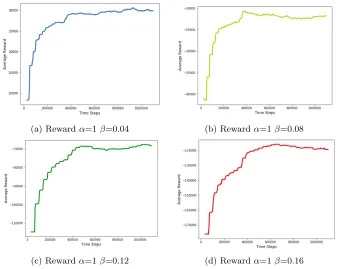
(a) Rewardα=1β=0.04 (b) Rewardα=1β=0.08

(c) Rewardα=1β=0.12 (d) Rewardα=1β=0.16

Figure 8: Reward of Different Parameters

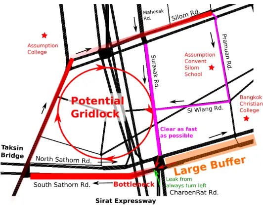
Figure 10: Potential Visual Policy of the Sathorn Road Network

The agent’s average vehicle throughput is shown in Figure9. It is expected that the order of the vehicle throughput at the end of 1 million agent steps would be in the inverse order of the weighted occupancy coefficient. This is because the more importance it places to the vehicle backlog from the β term, the less important the vehicle throughput provided by the α term is. At 800k agent steps, it is evident that the agent withβ = 0.04 has the highest throughput andβ = 0.08,0.12,0.16 in decreasing order. This shows the agent’s ability to be able to place importance in the concerning factors of the reward function.

An interesting insight could be seen in Figure11. All the parameter cases of the agent favor the lower jam length in the Surasak upstream lanes and place low importance in decreasing the South Sathorn jam length. An average Surasak jam length lower than 300 meters is observed in all cases after 600k agent steps, and South Sathorn jam length being over 500 meters after 400k agent steps. There is a slight change in this particular behavior when the importance in weighted occupancy term β is increased, allowing Surasak’s jam length to increase when comparing β = 0.04,0.08 andβ = 0.12,0.16. This policy is in agreement of the traffic police expert’s technique, using South Sathorn as the buffer zone to block the vehicles that could potentially enter the critical loop, while giving high priority to the Surasak upstream direction to be able to alleviate the potential gridlock as discussed in Section2.1. The policy could be further visualized in Figure10. It can be seen that congestion in the the upstream of the South Sathorn Road will likely not affect the current gridlock of interest, and with the large capacity of the link, the agent is able to treat it as a buffer to allow cars to fill in without allowing them to proceed to the bottleneck downstream link of the South Sathorn Road. On the other hand, the Surasak Road directly affects the potential gridlock that could happen and a high jam length could rapidly propagate the queue-length spillback to the other links. The Surasak Road should be taken care off quickly as a result.

(a) Surasak Jam Length (b) CharoenRat Jam Length

(c) South Sathorn Jam Length (d) North Sathorn Jam Length

Figure 11: Jam Length of the Approaching Lanes

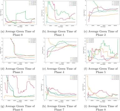
length divides into two courses of action: the two agents with the lower weighted occupancy coefficientβ= 0.04,0.08 allows the jam length in the CharoenRat direction to be at around 700 meters, while the other two agents with the higher weighted occupancy coefficientβ = 0.12,0.16 controls the jam length to be around 400 meters. This should be seen in conjunction with the average green time in Figure 12. The agent with higher weighted occupancy β = 0.12,0.16 does not allow the vehicles in the CharoenRat Road to fill up, as it would mean the increase of the total number of vehicles existent on the road. This is observed by the average green time of phases 3 and 8 in Figure12d and Figure 12i respectively. The agent with the higher weighted occupancyβ = 0.12,0.16 has an average green time on phases 3 and 8 at around 20 seconds, while the agents with the lower weighted occupancy β = 0.04,0.08 has much lower green time on these phases. Although the higher weighted occupancy agents favor the upstream of CharoenRat, the consistent average jam length of around 400 meters comes from the fact that CharoenRat is divided into two sections: the two leftmost lanes in the CharoenRat Road is always turn left and the two rightmost lanes in the CharoenRat Road is always turn right. Hence, the agent has no control over the vehicle leakage and the average jam length will always be existent if there is high queue length spillback in the downstream edge of South Sathorn and the flow of vehicles from the CharoenRat Road attempting to enter the critical loop exists.

(a) Average Green Time of Phase 0

(b) Average Green Time of Phase 1

(c) Average Green Time of Phase 2

(d) Average Green Time of Phase 3

(e) Average Green Time of Phase 4

(f) Average Green Time of Phase 5

(g) Average Green Time of Phase 6

(h) Average Green Time of Phase 7

(i) Average Green Time of Phase 8

Figure 12: Average Green Time of the 9 Phases

mean speed. The reasoning should be similar to what was previously mentioned, the Surasak Road being of crucial importance and the South Sathorn as an idle buffer. North Sathorn experiences a slight increase in mean speed and CharoenRat separates into two cases due to the shifted importance of the reward weights: the higher weighted occupancy β = 0.12,0.16 achieving a higher mean speed while the lower weighted occupancyβ = 0.04,0.08 achieves a lower mean speed.

(a) Surasak Mean Speed (b) CharoenRat Mean Speed

(c) South Sathorn Mean Speed (d) North Sathorn Mean Speed

Figure 13: Mean Speed of the Approaching Lanes

with limited sensory inputs in the traffic microsimulator SUMO. The Chula-SSS data with extended flows is used to trigger gridlock behavior as a base environment for the agent to learn. Results regarding the exploration with the reward being the weighted difference between the vehicle throughput and vehicle backlog (weighted occupancy) has been reported. The results show that the agent is able to derive insights and gridlock alleviation techniques similar to that of the traffic police experts even with no information about the whole gridlock state of all the critical looped road segments. However, the experiments reported on this paper are very limited with few hyperparameters tuning. Future works may continue to research further and do extensive ablation tests on the hyperparameters settings.

Future works can explore the agent’s reaction to the different constraints and limitations to the agent’s observability, and see how the agent changes its learning behaviors over each additional sensory input. This could prove to be useful in third world countries where sensors are scarce. Additionally, the reward function should also be worth further explorations for different combinations and formulation to increase the agent’s effectiveness when dense reward information signals are not available. The load factor for extended flows contributing to the gridlock loop can also be varied to observe the breakdown conditions and the optimal conditions with respect to the extent of the agent’s abilities for traffic light control.

This paper has demonstrated the capability of the agent to incur insightful actions for a larger problem with very limited knowledge. This capability of the agent can extend to further researches and potentially aid people to make more informed decisions for investment on sensors.

References

[1] Mart´ın Abadi, Ashish Agarwal, Paul Barham, Eugene Brevdo, Zhifeng Chen, Craig Citro, Greg S. Corrado, Andy Davis, Jeffrey Dean, Matthieu Devin, Sanjay Ghemawat, Ian Goodfellow, Andrew Harp, Geoffrey Irving, Michael Isard, Yangqing Jia, Rafal Jozefowicz, Lukasz Kaiser, Manjunath Kudlur, Josh Levenberg, Dan Man´e, Rajat Monga, Sherry Moore, Derek Murray, Chris Olah, Mike Schuster, Jonathon Shlens, Benoit Steiner, Ilya Sutskever, Kunal Talwar, Paul Tucker, Vincent Vanhoucke, Vijay Vasudevan, Fernanda Vi´egas, Oriol Vinyals, Pete Warden, Martin Wattenberg, Martin Wicke, Yuan Yu, and Xiaoqiang Zheng. TensorFlow: Large-scale machine learning on heterogeneous systems, 2015. Software available from tensorflow.org.

[2] Itamar Arel, Cuibi Liu, T. Urbanik, and A. G. Kohls. Reinforcement learning-based multi-agent system for network traffic signal control. IET Intelligent Transport Systems, 4(2):128–135, June 2010.

[3] Chaodit Aswakul, Sorawee Watarakitpaisarn, Patrachart Komolkiti, Chonti Krisanachantara, and Kittiphan Techakittiroj. Chula-sss: Developmental framework for signal actuated logics on sumo platform in over-saturated sathorn road network scenario. In Evamarie Wießner, Leonhard L¨ucken, Robert Hilbrich, Yun-Pang Fl¨otter¨od, Jakob Erdmann, Laura Bieker-Walz, and Michael Behrisch, editors, SUMO 2018- Simulating Autonomous and Intermodal Transport Systems, volume 2 of

EPiC Series in Engineering, pages 67–81. EasyChair, 2018.

[5] Greg Brockman, Vicki Cheung, Ludwig Pettersson, Jonas Schneider, John Schulman, Jie Tang, and Wojciech Zaremba. Openai gym, 2016.

[6] Samah El-Tantawy, Baher Abdulhai, and Hossam Abdelgawad. Multiagent reinforcement learning for integrated network of adaptive traffic signal controllers (marlin-atsc): Methodology and large-scale application on downtown toronto.IEEE Transactions on Intelligent Transportation Systems, 14(3):1140–1150, Sep. 2013.

[7] Meire Fortunato, Mohammad Gheshlaghi Azar, Bilal Piot, Jacob Menick, Ian Osband, Alex Graves, Vlad Mnih, Remi Munos, Demis Hassabis, Olivier Pietquin, Charles Blundell, and Shane Legg. Noisy Networks for Exploration. arXiv e-prints, page arXiv:1706.10295, Jun 2017.

[8] Juntao Gao, Yulong Shen, Jia Liu, Minoru Ito, and Norio Shiratori. Adaptive Traffic Signal Control: Deep Reinforcement Learning Algorithm with Experience Replay and Target Network.

arXiv e-prints, page arXiv:1705.02755, May 2017.

[9] Wade Genders and Saiedeh Razavi. Using a Deep Reinforcement Learning Agent for Traffic Signal Control.arXiv e-prints, page arXiv:1611.01142, Nov 2016.

[10] Matteo Hessel, Joseph Modayil, Hado van Hasselt, Tom Schaul, Georg Ostrovski, Will Dabney, Dan Horgan, Bilal Piot, Mohammad Azar, and David Silver. Rainbow: Combining Improvements in Deep Reinforcement Learning. arXiv e-prints, page arXiv:1710.02298, Oct 2017.

[11] Dan Horgan, John Quan, David Budden, Gabriel Barth-Maron, Matteo Hessel, Hado van Hasselt, and David Silver. Distributed Prioritized Experience Replay. arXiv e-prints, page arXiv:1803.00933, Mar 2018.

[12] Long ji Lin. Self-improving reactive agents based on reinforcement learning, planning and teaching.

InMachine Learning, pages 293–321, 1992.

[13] Leslie Pack Kaelbling, Michael L. Littman, and Anthony R. Cassandra. Planning and acting in partially observable stochastic domains. Artif. Intell., 101(1-2):99–134, May 1998.

[14] Eric Liang, Richard Liaw, Robert Nishihara, Philipp Moritz, Roy Fox, Ken Goldberg, Joseph E. Gonzalez, Michael I. Jordan, and Ion Stoica. RLlib: Abstractions for distributed reinforcement learning. InInternational Conference on Machine Learning (ICML), 2018.

[15] Pablo Alvarez Lopez, Michael Behrisch, Laura Bieker-Walz, Jakob Erdmann, Yun-Pang Fl¨otter¨od, Robert Hilbrich, Leonhard L¨ucken, Johannes Rummel, Peter Wagner, and Evamarie Wießner. Mi-croscopic traffic simulation using sumo. InThe 21st IEEE International Conference on Intelligent

Transportation Systems. IEEE, 2018.

[16] Volodymyr Mnih, Koray Kavukcuoglu, David Silver, Alex Graves, Ioannis Antonoglou, Daan Wierstra, and Martin Riedmiller. Playing Atari with Deep Reinforcement Learning. arXiv e-prints, page arXiv:1312.5602, Dec 2013.

[17] Volodymyr Mnih, Koray Kavukcuoglu, David Silver, Andrei A. Rusu, Joel Veness, Marc G. Belle-mare, Alex Graves, Martin Riedmiller, Andreas K. Fidjeland, Georg Ostrovski, Stig Petersen, Charles Beattie, Amir Sadik, Ioannis Antonoglou, Helen King, Dharshan Kumaran, Daan Wier-stra, Shane Legg, and Demis Hassabis. Human-level control through deep reinforcement learning.

Nature, 518(7540):529–533, February 2015.

[18] Philipp Moritz, Robert Nishihara, Stephanie Wang, Alexey Tumanov, Richard Liaw, Eric Liang, Melih Elibol, Zongheng Yang, William Paul, Michael I. Jordan, and Ion Stoica. Ray: A Distributed Framework for Emerging AI Applications. arXiv e-prints, page arXiv:1712.05889, Dec 2017. [19] Seyed Sajad Mousavi, Michael Schukat, and Enda Howley. Traffic Light Control Using

Deep Policy-Gradient and Value-Function Based Reinforcement Learning. arXiv e-prints, page arXiv:1704.08883, Apr 2017.

[20] Tom Schaul, John Quan, Ioannis Antonoglou, and David Silver. Prioritized Experience Replay.

arXiv e-prints, page arXiv:1511.05952, Nov 2015.

Foun-[24] Traffic and Transportation Department. Traffic statistics 2015. Technical report, Bangkok Metropolitan Administration, 2016.

[25] Hado van Hasselt, Arthur Guez, and David Silver. Deep Reinforcement Learning with Double Q-learning.arXiv e-prints, page arXiv:1509.06461, Sep 2015.

[26] Ziyu Wang, Tom Schaul, Matteo Hessel, Hado van Hasselt, Marc Lanctot, and Nando de Fre-itas. Dueling Network Architectures for Deep Reinforcement Learning. arXiv e-prints, page arXiv:1511.06581, Nov 2015.

[27] Axel Wegener, Michal Piorkowski, Maxim Raya, Horst Hellbr¨uck, Stefan Fischer, and Jean-Pierre Hubaux. Traci: An interface for coupling road traffic and network simulators. 11th

Communica-tions and Networking Simulation Symposium (CNS), 2008.

[28] Hua Wei, Guanjie Zheng, Huaxiu Yao, and Zhenhui Li. Intellilight: A reinforcement learning approach for intelligent traffic light control. InProceedings of the 24th ACM SIGKDD International

Conference on Knowledge Discovery and Data Mining, KDD ’18, pages 2496–2505, New York, NY,

USA, 2018. ACM.