Pi 2 waves simultaneously observed by Cluster and CPMN ground-based magnetometers near the plasmapause

www.ann-geophys.net/29/1663/2011/ doi:10.5194/angeo-29-1663-2011

© Author(s) 2011. CC Attribution 3.0 License.

Annales

Geophysicae

Pi 2 waves simultaneously observed by Cluster and CPMN

ground-based magnetometers near the plasmapause

H. Kawano1,2, S. Ohtani3, T. Uozumi2, T. Tokunaga1,*, A. Yoshikawa1,2, K. Yumoto2,1, E. A. Lucek4, M. Andr´e5, and the CPMN group6

1_{Department of Earth and Planetary Sciences, Kyushu University, Fukuoka, Japan} 2_{Space Environment Research Center, Kyushu University, Fukuoka, Japan} 3_{Johns Hopkins University, Applied Physics Laboratory, Laurel, USA}

4_{Space and Atmospheric Physics Group, Blackett Laboratory, Imperial College, London, UK} 5_{Swedish Institute of Space Physics, Uppsala, Sweden}

6_{http://denji102.geo.kyushu-u.ac.jp/denji/obs/cpmn/cpmn obs e.html}

*_{now at: Meiji Institute for Advanced Study of Mathematical Sciences, Kawasaki, Japan}

Received: 12 January 2011 – Revised: 13 June 2011 – Accepted: 1 August 2011 – Published: 28 September 2011

Abstract. We have analyzed an event on 14 February 2003 in which Cluster satellites and the CPMN ground magnetome-ter chain made simultaneous observations of a Pi 2 pulsation along the same meridian. Three of the four Cluster satellites were located outside the plasmasphere, while the other one was located within the plasmasphere. By combining the mul-tipoint observations in space and the mulmul-tipoint observations on the ground, we have obtained a detailedL-profile of the Pi 2 signatures, which has not been done in the past. In addi-tion, we have used a method called Independent Component Analysis (ICA) to separate out other superposed waves with similar spectral components. The result shows that the wave phase of the Pi 2 was the same up toL∼3.9 (corresponding to the plasmasphere), became earlier up toL∼4.1 (corre-sponding to the plasmapause boundary layer), and showed a delaying tendency up toL∼5.9 (corresponding to the plas-matrough). This systematic phase pattern, obtained for the first time by a combination of a ground magnetometer chain and multisatellites along a magnetic meridian with the aid of ICA, supports the interpretation that a Pi 2 signal propagated from a farther source and reached the plasmasphere. Keywords. Magnetospheric physics (Magnetotail boundary layers; MHD waves and instabilities; Plasmasphere)

Correspondence to: H. Kawano ([email protected])

1 Introduction

The Pi 2 pulsation is the transient wave phenomenon ob-served in space and on the ground at the start time of a mag-netospheric substorm (e.g. Olson, 1999) or a pseudo-breakup (Hsu and McPherron, 2007). Pi 2 has its period in the range of 40–150 s, typically has a damping-type waveform, and typically continues for a few minutes to∼10 min.

There exist many publications as regards the source region and propagation of Pi 2. Among them, Uozumi et al. (2004, 2007) statistically analyzed Pi 2’s observed at high-latitude ground magnetometers belonging to the Circum-pan Pacific Magnetometer Network (CPMN) (Yumoto and the 210MM Magnetic Observation Group, 1996; Yumoto and the CPMN Group, 2001) to estimate the source region of Pi 2 to be lo-cated in space at 9 Re (from the geocenter) and 22.5 MLT; they assumed that Pi 2 propagated as fast-mode and Alfven waves from the source region down to the ground high lat-itudes, and made model calculations that best-matched the observed time lags among the ground stations they used. Chi et al. (2009) analyzed four Pi 2’s observed at a meridian chain of ground magnetometers located at 300–330◦magnetic lon-gitudes in the north-American continent. For each Pi 2, they fit their Pi 2-propagation model to estimate the onset posi-tion; as a result, they obtainedX∼ −20RE.

There remain arguments about the outer boundary of the cavity mode oscillation, but a popular idea is that the plasma-pause is the outer boundary: Takahashi et al. (2003) per-formed a detailed statistical analysis of the magnetic and electric field data from the CRRES satellite, and concluded that the node of the cavity mode is located near the plasma-pause.

The above-cited source region of Pi 2 is located outside the plasmasphere; thus, a question has been how the cavity mode is excited by the outside source. A scenario has been that an impulse from the source region propagates inward and hits the magnetospheric cavity (e.g. Yeoman and Orr, 1989). However, the actual process of this hitting was not observed well in space in the 20th century, because a single satellite was not good enough to separate out the temporal effects from the spatial effects near the plasmapause. The 2000 launch of Cluster, consisting of four identical satellites (Escoubet et al., 2001), provided for the first time in his-tory chances for simultaneously observing the region near the plasmapause by multiple satellites.

Collier et al. (2006) were the first to analyze a case in which Cluster satellites were located near the plasmapause during a Pi 2 event; three of the four satellites were located within the plasmasphere (CL1, CL2, and CL4 atL=4.7, 4.5, and 4.6) while the fourth (CL3 atL=6.6) was located at or just outside the plasmapause. As a result of the analysis they found in the data of the three satellites in the plasmasphere evidence for the standing wave in both the radial and field-aligned directions, strongly indicative of the cavity mode. On the other hand, the magnetic field perturbation observed at CL3 preceded the activity at the other three satellites (lo-cated within the plasmasphere), which may be attributed to the time interval required for inward radial propagation of the Pi 2 signal; though, they also stated that the perturbation at CL3 was highly irregular, quite distinct from those at the other three satellites. They stated that one cannot exclude the possibility that the Pi 2 event at CL3 was masked by other waves with similar spectral content.

In this paper we have also found a Pi 2 event for which Cluster satellites were located near the plasmapause; we also analyze data from the four Cluster satellites. In addition, as a new feature of this paper, we also use simultaneously obtained data at a ground magnetometer chain: the Cluster magnetic footprints were located close (in longitude) to the meridian of the ground magnetometers at the time of the Pi 2 event, and thus, by field-aligned mapping the Cluster data to the ground and analysing them along with the data from the ground magnetometer chain, we will be able to understand theLdependence of the event in a systematic manner. Also, we will use a method called Independent Component Anal-ysis (ICA) to separate out other waves with similar spectral content.

2 Data

2.1 Cluster spacecraft

Cluster consists of four identical satellites, which were launched in 2000 (Escoubet et al., 2001). The four satel-lites were kept close to each other in space. The orbital planes of the satellites were also close to each other and the normal vectors of the orbital planes were fairly perpendic-ular to the earth’s axis. At the launch, the geocentric dis-tances of the apogees (perigees) of the Cluster spacecraft were∼20(∼4)RE; these small perigees enabled Cluster to

sometimes enter the plasmasphere, and the event of this pa-per is such an example.

In this paper we show the magnetic field data measured by the FGM instrument (Balogh et al., 2001) and the spacecraft potential data measured by the EFW instrument (Gustafsson et al., 1997), both on board the Cluster spacecraft. The data were retrieved from the Cluster Active Archive (http://caa. estec.esa.int/caa/) with time resolution of 0.2 s (4 s) for the magnetic field data (spacecraft potential data).

For the magnetic field data analysis of Pi 2 waves, we will use mean-field-aligned (MFA) coordinates (e.g. Takahashi et al., 2001; Collier et al., 2006). In this system,ezis in the

di-rection of the mean magnetic field, which is defined by 150-s moving averages of the 0.2-s magnetic field data;ey, is

par-allel toez×r, whereris the vector from the geocenter to the

satellite; andexis set so as to complete the (ex,ey,ez)triad.

Finally, the 0.2-s data in MFA coordinates are averaged over 3sec and will be used for the Pi 2 analysis of this paper. 2.2 CPMN ground magnetometers

For comparisons with the above-stated Cluster data, we use simultaneously observed ground magnetometer data from the Circum-pan Pacific Magnetometer Network (CPMN) (Yu-moto and the 210MM Magnetic Observation Group, 1996; Yumoto and the CPMN Group, 2001), mainly run by the Space Environment Research Center (SERC), Kyushu Uni-versity, Japan. We use 3-sH-component data from CPMN stations along the 210◦magnetic meridian (MM). The loca-tions of the staloca-tions are listed in Table 1. For each ground station, the table shows its geographic (GEO) coordinates, AACGM (Baker and Wing, 1989) coordinates, andL-value calculated by using the equation L=1/(cosλ)2 where λ

refers to the AACGM latitude. Table 1 also shows the lo-cation information of the four Cluster satellites.

3 Data analysis

Table 1. Geographic and geomagnetic coordinates of the CPMN ground stations and the Cluster satellites used in this paper. Geographic

coordinates of the Cluster satellites are those of the footprints of the satellites at 14:02:02 UT on 14 February 2003, calculated by using the Tsyganenko 96 model. Geomagnetic coordinates of the ground stations and the Cluster footprints are calculated by using AACGM. The

L-value is calculated by using the equationL=1/(cosλ)2whereλrefers to the AACGM latitude. In-situ locations of the Cluster satellites, in geocentric distance (r)and geomagnetic coordinates (latitude and longitude), are also shown in the rightmost three columns. See the text for more details.

CPMN or Cluster footprints Cluster in-situ

Geographic AACGM L r geomagnetic

lat long lat long lat long

TIK 71.59 128.78 65.76 196.87 5.93

CL1 69.82 178.74 65.46 234.52 5.80 4.82 29.70 235.65 CHD 70.62 147.89 64.79 212.19 5.51

CL2 67.72 178.26 63.18 235.75 4.91 4.46 24.57 236.77 CL4 65.15 178.17 60.41 237.27 4.10 4.07 16.90 238.18 ZYK 65.75 150.78 59.74 216.91 3.94

CL3 64.28 180.76 59.72 239.59 3.93 4.28 −2.76 240.93 MGD 59.97 150.86 53.60 218.94 2.84

PTK 52.94 158.25 46.18 226.21 2.09 GAM 13.58 144.87 5.82 215.61 1.01 BSV −25.54 139.21 −36.01 213.09 1.53 ADL −34.67 138.65 −46.13 213.83 2.08

-4 -2 0 2 4

-4 -2 0 2 4

ZGSE [Re]

XGSE [Re] -4

-2 0 2 4

YGSE [Re]

CL1 CL2 CL3 CL4

-4 -2 0 2 4

YGSE [Re]

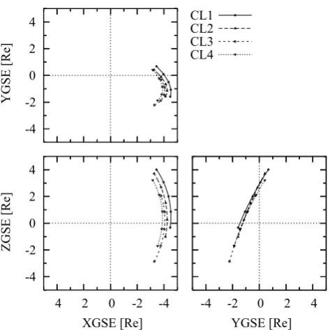
Fig. 1. Shows the orbital segments of the Cluster satellites for

the interval 13:00–15:00 UT on 14 February 2003, in GSE co-ordinates. The orbital information was taken from the SSCweb (http://sscweb.gsfc.nasa.gov/). All the satellites moved upward in the bottom two panels. Different symbols are plotted for different satellites, at 13:00, 13:30, 14:00, 14:30, and 15:00 UT.

Rightmost three columns of Table 1 list the locations of the Cluster satellites in space at 14:02:02 UT, in terms of the geocentric distance, geomagnetic (MAG) latitude, and MAG longitude.

For each Cluster satellite, Table 1 also shows the loca-tion of its footprint, field-aligned traced by using the Tsy-ganenko 96 (T96) model (TsyTsy-ganenko, 1996). The L -value of the Cluster footprint, shown in the table, is calcu-lated by using the equationL=1/(cosλ)2 whereλ refers to the AACGM latitude of the footprint. The T96 model parameters are set as follows: DP = 3.4 nPa, Dst =−3 nT, IMFBy= 8.7 nT, and IMFBz=−0.7 nT; these values were

measured by the ACE spacecraft (http://www.srl.caltech.edu/ ACE/ASC/index.html) except that Dst originally came from NSSDC Kyoto (http://wdc.kugi.kyoto-u.ac.jp/). In more detail, since the magnetosphere responds relatively gradu-ally to changes in these parameters, we have used OMNI hourly averages of these quantities available on CDAWeb (http://cdaweb.gsfc.nasa.gov/); we have averaged the data corresponding to two intervals 13:00–14:00 UT and 14:00– 15:00 UT (in OMNI data, the propagation lag from ACE to the magnetosphere is already taken into account). We note in Table 1 that the footprints of the Cluster satellites are close to the CPMN stations in longitude (see AACGM long).

-40 -20 0

CL1

-40 -20 0

CL2

-40 -20 0

CL3

-40 -20 0

CL4

7 8 9 10 11 12 13 14 15 16 17 18 19 20 21

Feb 14, 2003 [hour UT]

ASPOC ASPOC

SP

- [Volt]

Fig. 2. Shows the negative of the spacecraft potential (SP−) mea-sured by the EFW experiment on board the Cluster spacecraft (from top, Cluster CL1, CL2, CL3, and CL4). The vertical line is drawn at the onset time of the Pi 2 analyzed in this paper (14:02:02 UT). See the text for more details.

SP−_{becomes flat near zero. The ASPOC intervals for CL3} and CL4 are shown by superposed horizontal lines in Fig. 2 (ASPOC of CL1 and CL2 was not activated during the inter-val of the figure).

Figure 2 shows that, for all the four satellites, the SP−’s were large near the beginning and the end of the time inter-val of the figure; for these interinter-vals the satellites were lo-cated within the magnetosheath-solar wind. Next to these magnetosheath-solar wind intervals, the satellites were lo-cated within the tail lobe-polar cap, thus the SP−’s were much smaller.

Near the centre of Fig. 2, the SP−’s were large for all the satellites; for these intervals the satellites were located within the plasmasheet-plasmasphere. In particular, the rectangu-lar bumps (∼13:10 UT for CL1, 13:00–13:40 UT for CL2, 13:50–14:25 UT for CL3, and 13:10–14:00 UT for CL4) likely correspond to the entries of the satellites into the plas-masphere when they were near their perigees; this interpre-tation is consistent with the region information we can ob-tain from the quick-look energy-time ion spectrograms from the CIS instrument onboard Cluster (R`eme et al., 2001) (not shown here) (The quicklooks are found at http://cluster.cesr. fr:8000/public/spectro/index.php?vue=SCI).

The vertical line in Fig. 2 marks the Pi 2 onset time (14:02:02 UT; discussed below by using Fig. 3). At this Pi 2 onset time, CL1, CL2, and CL4 were located outside the plasmasphere while CL3 was located inside the plasmas-phere, as shown by the above-mentioned bumps.

Figure 3 is an overview plot of the ground Pi 2 signatures; shown are theH-component data from the CPMN stations listed in Table 1, bandpass filtered with the Pi 2 period range

13:30 13:40 13:50 14:00 14:10 14:20 14:30 -2

-2 -20 0 20

-50 0 50

-10 0 10

-2 0 2

-2 0 2

-1 0 1

0 2

0 2 TIK L=5.93

CHD L=5.51

ZYK L=3.94

MGD L=2.84

PTK L=2.09

GAM L=1.01

BSV L=1.53S

ADL L=2.08S

H Comp. UT (2003/02/14)

Fig. 3. Overview plot of the ground Pi 2 signatures; shown are the

H-component data from the CPMN stations listed in Table 1, band-pass filtered with the Pi 2 period range (40–150 s). The Pi 2 onset time, 14:02:02 UT, determined by visual inspection of the GAM data, is shown by the vertical line. See the text for more details.

-400 -300 -200 -100

TIK (L=5.93)

13:30 13:40 13:50 14:00 14:10 14:20 14:30

-10 -5 0 5 10

GAM (L=1.01)

H Component UT on 2003/02/14

Fig. 4. Shows the raw data plot of theH-component magnetometer data from the CPMN stations TIK and GAM. See Table 1 for their locations. The vertical line is drawn at the onset time of the Pi 2 analyzed in this paper (14:02:02 UT). See the text for more details.

(40–150 s). The Pi 2 onset time, 14:02:02 UT, determined by visual inspection of the GAM data, is shown by the vertical line. The Pi 2 signal is clearly identified at ZYK through ADL.

-15 -10-5 0 5 10 15 Bx -15 -10-5 0 5 10 15 By

14:00 14:05 14:10 -15 -10-5 0 5 10 15 Bz UT (2003/02/14) -3 -2 -10 1 2 3 Bx -3 -2 -10 1 2 3 By

14:00 14:05 14:10 -3 -2 -10 1 2 3 Bz UT (2003/02/14) -0.5 0 0.5 Bx -0.5 0 0.5 By

14:00 14:05 14:10 -0.5 0 0.5 Bz UT (2003/02/14) -0.2 0 0.2 0.4 Bx -0.2 0 0.2 0.4 By

14:00 14:05 14:10 -0.2 0 0.2 0.4 Bz UT (2003/02/14) CL1 CL2 CL3 CL4

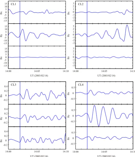
Fig. 5. Shows the bandpass-filtered (40–150 s) magnetic field data

of the Pi 2 of this paper observed by CL1 (top left), CL2 (top right), CL3 (bottom left), and CL4 (bottom right). The magnetic field vec-tor is expressed in the mean-field-aligned (MFA) coordinates. The Pi 2 onset time (14:02:02 UT) is shown by the vertical lines. See the text for more details.

identifiable positive bay started at GAM (located at low lat-itudes). We also note that LANL geosynchronous satellite 1994-084 (which was located at∼23:36 LT at 14:02 UT) ob-served a signature of a low-energy particle injection (not shown here) (the 1994-084 data are available at CDAWeb: http://cdaweb.gsfc.nasa.gov/). Thus, we can say that this Pi 2 took place at the start time of a substorm.

Figure 5 shows the bandpass-filtered (40–150 s) magnetic field data from the four Cluster satellites for the 10-min inter-val including the Pi 2 introduced above. The magnetic field vector is expressed in the MFA coordinates. Note that the vertical axis range is different from satellite to satellite, al-though it is the same for the three subpanels (showingBx, By, andBz) in each panel. From this figure one can see that Byis generally larger thanBxandBzin amplitude, and that

the waveforms looks different from satellite to satellite and from component to component.

To study the relation between such Cluster signatures and the CPMN ground signatures, we have first performed the correlation analysis, as follows. First, by visual inspection, we have selected the interval during which the Pi 2 in ques-tion was significant at all the four Cluster satellites. The re-sultant interval is 14:01:30–14:09:37 UT (Cluster data plots

-10 0 10 -20 0 20 -5 0 5 -5 0 5 -1 0 1 -5 0 5 -0.5 0 0.5 -2 0 2 -2 0 2 -1 0 1 -2 0 2 -2 0 2

14:02 14:03 14:04 14:05 14:06 14:07 14:08 14:09

CL B_y and CPMN H UT (2003/02/14) CHD L=5.51 MGD L=2.84 PTK L=2.09 GAM L=1.01 BSV L=1.53S ADL L=2.08S CL2 L=4.91 CL4 L=4.10 CL3 L=3.93 ZYK L=3.94 CL1 L=5.80 TIK L=5.93

Fig. 6. Shows, in the order ofL, the bandpass-filtered data of CPMN groundHand ClusterBy(eastward component in the MFA

coordinates). The period range of the bandpass filter is 40–150 s. The vertical line is meant as a guide, and is plotted so as to run through a minimum at MGD-ADL. See the text for more details.

for this interval will be shown below); the number of 3-s-resolution Cluster data in this interval is 163.

We have then calculated the coherence between GAMH

and CL Bx, the coherence between GAMH and CL By,

and the coherence between GAM H and CL Bz for each

of the four Cluster satellites, for the interval 14:01:30– 14:09:37 UT; here we are using the data from GAM, located near the magnetic equator, as the reference ground data. The coherence is calculated by using FFT, with a data window of 128 datapoints (i.e. 384 s) slided by every eight datapoints. From thus obtained results, we use the coherence at a pe-riod of 96 s, at which the GAMH data during the interval 14:01:30–14:09:37 UT had the maximum power.

Thus obtained coherence was larger than 0.6 for CL4By,

CL3By, CL3Bx, CL1Bx, CL1By, and CL2By; that is, these

six components are regarded as significantly correlated with GAMH. (This threshold 0.6 is often used in Pi 2 studies; see, e.g. Takahashi et al., 1995.) It is to be noted that, at all the four Cluster satellites, theBycomponent is significantly

correlated with the groundHcomponent. On the other hand, only two satellites show significant correlation inBx, and no

satellite shows significant correlation inBz. In this paper we

the four Cluster satellites, and for this purposeBxandBzare

insufficient. Thus, in this paper we concentrate onBy.

Figure 6 shows the bandpass-filtered data of CPMN ground H and Cluster By, in the same time frame as that

used for the above-stated coherence analysis (i.e. 14:01:30– 14:09:37 UT), in the order ofL. The vertical line is meant as a guide, and is plotted so as to run through a minimum at MGD-ADL. It is to be noted that CL3Byis reversed in

its sign; it is made so because only CL3 was in the South-ern Hemisphere (ZMAG= −0.2 Re on 14:02 UT) while the

other three Cluster satellites were in the Northern Hemi-sphere (ZMAG=2.4, 1.9, and 1.2 for CL1, CL2, and CL4).

In Fig. 6, the low-latitude stations (MGD-ADL) show co-herent perturbations: this feature has frequently been re-ported in publication and has often been regarded as a man-ifestation of the cavity mode (e.g. Yumoto and the CPMN group, 2001; Takahashi et al., 2003). It is to be noted that the plasmapause was located between CL4 and CL3 (see Fig. 2); thus, MGD-ADL are all likely to have been within the plas-masphere. On the other hand, the waveforms at higher lati-tudes look very different from those at low latilati-tudes, which complicates further analysis. Here we expect that the higher-latitude data include signals similar to those at low higher-latitudes, but superposed signals complicate the higher-latitude data; then, to extract the common part, we use the method called the Independent Component Analysis (ICA), which is ex-plained below.

When signals having different characteristics are mixed, each signal is naturally regarded as being independent from the others. Thus, ICA uses a statistical-mathematics ap-proach to separate out different signals included in a time-series by maximizing the independence of each signal. ICA has been proven to be useful, for example, for cases in which one wants to separate out several speakers’ voices when they speak at the same time (examples are found in the textbook by Hyv¨arinen et al., 2001). As the computer algorithm of ICA, in this paper we use FastICA (Hyv¨arinen, 1999) the software of which is found at http://www.cis.hut.fi/projects/ ica/fastica/. FastICA uses the algorithm called “fixed-point algorithm” to maximize the independence of signals to be separated out. We also note that Tokunaga et al. (2007) ap-plied FastICA to ground magnetometer data of a Pi 2 event for the first time in space physics.

Figure 7 shows the result of applying ICA to the bandpass-filteredH-component data from the eight CPMN stations (as shown in Fig. 6) and bandpass-filteredBx,ByandBzfrom

the four Cluster satellites (i.e. applying ICA to 8+3×4=20 timeseries) in the same time frame as that used for the above-stated coherence analysis (i.e. 14:01:30–14:09:37 UT). Here we are using two independent components (IC’s) that well reproduce the waveforms of low- to mid-latitude groundH

(ZYK-ADL); each of the two IC’s (not shown) has a wave-form similar to the observed Pi 2, and the phases of the two IC’s are different from each other, so that the combination of the two IC’s can express the time lag between different

-0.2 0 0.2 CL3 L=3.93

-5 0 5 ZYK L=3.94

-20 0 20 CL1 L=5.80

-10 0 10 TIK L=5.93

-2 0 2

-1 0 1

-1 0 1

-2 0 2

-2 0 2

-1 0 1

-10 1

-2 0 2

14:02 14:03 14:04 14:05 14:06 14:07 14:08 14:09 CL B_y and CPMN H UT (2003/02/14) CHD

L=5.51

MGD L=2.84 PTK L=2.09 GAM L=1.01 BSV L=1.53S ADL L=2.08S CL2 L=4.91 CL4 L=4.10

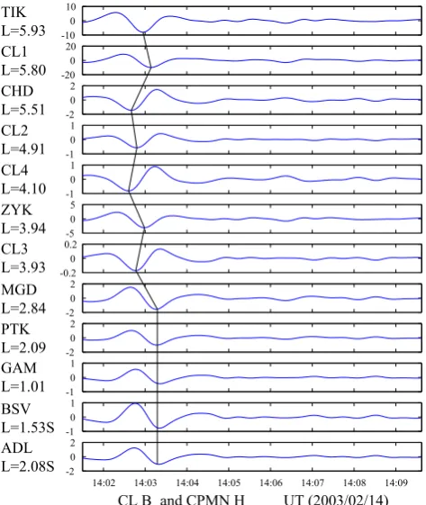
Fig. 7. Shows the result of applying ICA to the bandpass-filtered

H-component data from the eight CPMN stations (as shown in Fig. 6) and bandpass-filteredBx, Byand Bzfrom the four

Clus-ter satellites. Superposed line segments pass through a minimum in each timeseries data. See the text for more details.

datasets (such as that between ZYK and MGD, which is clear in Fig. 6). It is to be noted that Fig. 7 shows onlyByfrom

the four Cluster satellites, even though ICA was also applied toBxandBz at once (in order to best extract the common

feature in the available data with ICA). Superposed line seg-ments pass through a minimum in each timeseries data.

If we try to understand the observed phase pattern in terms of the Pi 2 propagation effect, we have to take into account the propagation time from Cluster to the ground along the magnetic field line. To calculate it, we use the procedure of Uozumi et al. (2000, 2007): we assume a cold plasma consisting of hydrogen ions and electrons, use the Tsyga-nenko 96 model for the magnetic field, use the model of Car-penter and Anderson (1992) for the equatorial plasma den-sity, and use the power-law model for the field-aligned dis-tribution of the plasma densityn, i.e.n(r)=neq(r/req)−p,

wherer is the geocentric distance of any point on a field line, reqisr on the equatorial plane,neq isn there, andp

is set to 3 (4) inside (outside) the plasmapause (Takahashi and Anderson, 1992). By using these models we have cal-culated the Alfven velocity (VA) distribution along the field

14:02 14:03 14:04 14:05 14:06 14:07 14:08 14:09 CL By and CPMN H UT (2003/02/14) -0.2

0 0.2 CL3 L=3.93

-5 0 5 ZYK L=3.94

-20 0 20 CL1 L=5.80

-100 10 TIK L=5.93

-2 0 2

-1 0 1

-1 0 1

-2 0 2

-2 0 2

-1 0 1

-1 0 1

-2 0 2 CHD L=5.51

MGD L=2.84 PTK L=2.09 GAM L=1.01 BSV L=1.53S ADL L=2.08S CL2 L=4.91 CL4 L=4.10

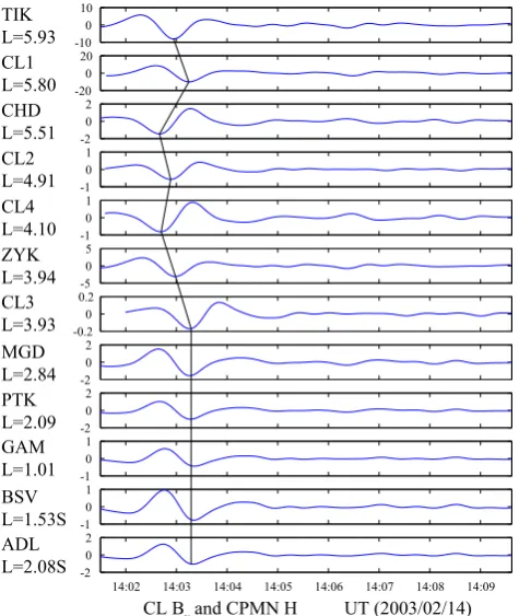
Fig. 8. The same as Fig. 7 except that the Cluster data are shifted

in time so as to correct for the field-aligned propagation time from the position of each satellite to the ground. See the text for more details.

the ground. Thus obtained travel times are 6.9 s, 5.4 s, 29.5 s, and 5.4 s for CL1, CL2, CL3, and CL4; these times are ex-pected to be the time lag from the in-situ observation time at Cluster to the expected observation time at the ground foot-print. If we apply this time shift to the Cluster data in Fig. 7, the result is that shown in Fig. 8. The time shift is small for CL1, CL2, and CL4, because they were located within the plasmatrough whereVAis generally high; on the other hand

the time shift is pretty large (about 30 s) for CL3 because CL3 was located within the plasmasphere whereVAis lower.

As a result of the time shift, the latitude dependence of the Pi 2 phase in Fig. 8 is more systematic than in Fig. 7; first let us recall that, as shown in Fig. 2, CL3 was within the plasmasphere while CL4 was outside the plasmapause. Then, Fig. 8 shows that the phase was almost constant within the plasmasphere, and that the phase was earlier just outside the plasmapause (CL4, CL2, and CHD). At largerL (CL1 and TIK) the phase was later. These features will be further discussed in the next section.

0 2 4 6 8 10

2S 0 2 4 6

CL1

CL2 CL3CL4

L-value

Pi 2 amplitude (with ICA) [nT]

Fig. 9. Visualizes the wave amplitudes shown in Figs. 7 and 8. The

horizontal axis is theL-value and the vertical axis is the half of the maximum peak-to-peak amplitude shown in Figs. 7 and 8. Filled circles (labelled) correspond to Cluster, while the open squares (not labelled) correspond to the CPMN ground stations.

4 Discussion and summary

For the Pi 2 event of this paper, only the By (eastward)

component showed perturbations coherent with the ground

H-component perturbations at all the four Cluster satellites; because the purpose of this paper is to study the relations be-tween simultaneous observations by Cluster multisatellites and multiple ground magnetometers, in this paper we have concentrated on theBycomponent.

One may think that the Bx (radial) component in

space should have a good correlation with the ground

H-component for cavity mode-type perturbations; it is a topic of future research to identify the reason why it was not such for our event, but we note that Collier et al. (2006) re-ported another case of Pi 2 observed by Cluster, in which CL2 and CL4 within the plasmasphere observed significant oscillations inBy(see their Fig. 4); Collier et al. (2006)

at-tributed this feature to coupling between the cavity mode and the toroidal mode, which could take place if the cavity mode had a non-zero azimuthal wave number. Perhaps our event also had a non-zero azimuthal wave number, and the big por-tion of the cavity mode wave energy was put into the oscilla-tions in the azimuthal direction.

to the auroral latitudes. On the other hand, if we look at Clus-ter, the Pi 2 amplitude at CL1 was about 10 times larger than that at ground low latitudes (i.e.∼1 nT at GAM and BSV), the Pi 2 amplitudes at CL2 and CL4 were comparable to that at the ground low latitudes, and the Pi 2 amplitude at CL3 was about 1/10 of that at the ground low latitudes.

If we try to sort out these amplitudes at Cluster in terms of the above-stated latitude dependence of the amplitude, CL1 is consistent because the amplitude at CL1 (L=5.80) was similar to that at the adjacent (in terms of theLvalue) higher-latitude station TIK (L=5.93). On the other hand, the am-plitudes at CL2, CL4 and CL3 (especially CL3) were smaller than those at the adjacent (inL)ground stations in the figure (i.e. CHD (L=5.51) and ZYK (L=3.94)), not apparently consistent with the above-stated latitude dependence. For CL4 and CL3, we think the small amplitudes were caused because CL4 and CL3 were located at low latitudes in space (16.90◦_and−2.76◦_{in latitude; see Table 1). That is, if the} observed Pi 2 was caused by fundamental mode-type oscil-lations of the field lines, thenByin space is expected to have

been small near the equator which corresponded to the antin-ode of the field-line oscillations.

On the other hand, the small amplitude at CL2 (L=4.91) about half of that at nearby ground station CHD (L=5.51), is rather difficult to explain, because CL2 was located at 24.57◦in latitude in space (see Table 1), i.e. at pretty much high latitude. We note that CL2 shows the data for which the waveforms in Figs. 6 and 7 are the most different (that is, the wave amplitude in Fig. 6 is at maximum in the latter half of the time interval of the figure), and that the maximum ampli-tude at CL2 in Fig. 6 is comparable to that at CHD, which also shows a fairly large difference in the waveform between Figs. 6 and 7 so that its maximum amplitude in Fig. 7 is less than half of that in Fig. 6. Our speculation here is that the area (in space) near CL2 and CHD (L∼5) was associated with active wave-mode conversion from Pi 2 to some other type, so that the wave energy of Pi 2 was lost to some extent at CL2 and CHD.

We saw above that, by taking into account the field-aligned Alfven-wave travel time from Cluster to the ground (Fig. 8), the latitude-phase relation of Pi 2 becomes more systematic than otherwise (Fig. 7). From this we think that the data cor-responding to the plasmatrough (CL4 (L=4.10) and larger

L)were caused by the earthward propagation of the Pi 2 sig-nal. We also note that Uozumi et al. (2009) explained their observations of Pi 2’s at TIK and CHD in terms of the Pi 2 wave propagation.

Past studies show that the source region of Pi 2 is usually field-aligned mapped to the ground more poleward than TIK (L=5.93). Then, at first glance, the delay in the phase at CL1 and TIK from CHD-CL4 may appear to contradict with the interpretation in terms of the Pi 2 propagation; however, in fact it does not, as follows.

Figure 1a of Uozumi et al. (2007) and Fig. 2a of Chi et al. (2009) illustrate how the Pi 2 signal propagates from the

source region to the ground: for the L of CL1 and CHD, the travel path is such that the Pi 2 signal first propagates in the equatorial plasmasheet toward the Earth as the fast-mode wave, and when the signal reaches the field line running through the ground station, it is mode-converted from the fast mode to the Alfven mode and propagates along the field line toward the Earth. Figure 2b of Chi et al. (2009) illustrates that the Alfvenic field-aligned travel time decreases sharply with decreasingL; it is so becauseVAsharply increases with

decreasingLin the trough (see, e.g. Fig. 1, top panel of Fujita et al., 2001 for illustration). This is the reason why the Pi 2 signal in the mid-latitude trough reaches the ground faster than the Pi 2 signal in the higher-latitude trough. (It is to be noted that the majority of the Alfvenic field-aligned travel time is spent near the equatorial plasmasheet, becauseVA

in-creases very quickly as the Alfven wave field-aligned propa-gates from the equator toward higher latitudes in space; see, e.g. Fig. 1, bottom panel of Fujita et al. (2001) for illustra-tion. This is the reason why the estimated field-aligned travel time is not significant for CL1, CL2, and CL4 in Fig. 8; these satellites were located off the equator.)

In Fig. 8, the phase delay is less for TIK than for CL1, although a natural expectation is the opposite (as explained above). We think this happened due to azimuthal propaga-tion of the Pi 2 signal with TIK located significantly west-ward of the other observation points (see Table 1). That is, at the event time, TIK was located at 22.6 LT while the other ground stations were located at 23.3–24.6 LT. If the Pi 2 source region of our event was near 22.5 MLT which is the statistical average for Pi 2 observed by CPMN (Uozumi et al., 2004), it is expected that the eastward propagation of the Pi 2 signal from the source region made TIK observe the Pi 2 faster than the other stations. Similar azimuthal propagation effect was reported by Uozumi et al. (2004).

In Fig. 8, the monotonic delay in phase from CL4 to CL3 is likely to have been caused by the Pi 2 propagation in the plasmapause boundary layer whereVAsharply decreases

with decreasing L (see the region near L=5 in Fig. 1 of Lee and Lysak, 1999 or in Fig. 1 (top) of Fujita et al., 2001 for illustration). The plasmasphere, including CL3 and the lower-latitude ground stations (MGD-ADL), was hit by this Pi 2 signal, and the cavity mode would have formed in the plasmasphere, as reported in many past papers. As expected at the beginning of this work, we could confirm this propa-gation and hitting process by the combination of the Cluster multisatellites in space and the CPMN ground magnetometer network, and with the aid of ICA to separate out other waves with spectral content similar to Pi 2.

travel time from radial travel time of Pi 2. For example, Uozumi et al. (2000) statistically showed that Pi 2 signals propagating within the plasmasphere were observed earlier at smallerLon the ground (see their Fig. 3), unlike the one shown in this paper, and successfully explained it by their model cited above. On the other hand for the event of this paper, the phase is very coherent within the plasmasphere, but it might also be explained with a propagation model with different model parameters.

As a multisatellite observation within the plasmasphere, Collier et al. (2006) presented a case in which CL1, CL2, and CL4 were located within the plasmasphere, and they found evidence for the cavity mode. Since their Pi 2 oscil-lated about three times in its wave packet while our Pi 2 (its common part identified by ICA) oscillated only about once (Fig. 6–8), there may be an argument such a short wave is not enough to establish the standing oscillation of the cav-ity; however, we note Fujita et al. (2002) simulated a Pi 2 by inputting a single pulse in their simulation code, and they showed that the entire plasmasphere started to oscillate in the cavity mode very fast. Thus, the number of oscillations of Pi 2 may not be relevant for the establishment of a cav-ity wave. A reasonable extension of this earlier study by Collier et al. (2006) would be to analyze cases in which a Pi 2 is simultaneously monitored in the plasmasphere by a ground magnetometer chain and multisatellites along the same meridian, to distinguish the field-aligned travel time from the radial travel time with observations; it is a topic of future research.

Acknowledgements. Work at JHU/APL was supported by NASA

grants NNX07AG07G and NNX09AF46G. The FastICA package is free software under copyright 1996–2005 by Hugo G¨avert, Jarmo Hurri, Jaakko S¨arel¨a, and Aapo Hyv¨arinen.

Topical Editor I. Daglis thanks A. Collier and another anony-mous referee for their help in evaluating this paper.

References

Baker, K. B. and Wing, S.: A new magnetic coordinate system for conjugate studies at high latitudes, J. Geophys. Res., 94(A7), 9139–9144, 1989.

Balogh, A., Carr, C. M., Acu˜na, M. H., Dunlop, M. W., Beek, T. J., Brown, P., Fornacon, H., Georgescu, E., Glassmeier, K.-H., Harris, J., Musmann, G., Oddy, T., and Schwingenschuh, K.: The Cluster Magnetic Field Investigation: overview of in-flight performance and initial results, Ann. Geophys., 19, 1207–1217, doi:10.5194/angeo-19-1207-2001, 2001.

Carpenter, D. L. and Anderson, R. R.:, An ISEE/Whistler model of equatorial electron density in the magnetosphere, J. Geophys. Res., 97, 1097–1108, 1992.

Chi, P. J., Russell, C. T., and Ohtani, S.: Substorm onset timing via traveltime magnetoseismology, Geophys. Res. Lett., 36, L08107, doi:10.1029/2008GL036574, 2009.

Collier, A. B., Hughes, A. R. W., Blomberg, L. G., and Sut-cliffe, P. R.: Evidence of standing waves during a Pi2

pulsa-tion event observed on Cluster, Ann. Geophys., 24, 2719–2733, doi:10.5194/angeo-24-2719-2006, 2006.

Escoubet, C. P., Fehringer, M., and Goldstein, M.:

Introduc-tion The Cluster mission, Ann. Geophys., 19, 1197–1200,

doi:10.5194/angeo-19-1197-2001, 2001.

Fujita, S., Mizuta, T., Itonaga, M., Yoshikawa, A., and Nakata, H.: Propagation property of transient MHD impulses in the magnetosphere-ionosphere System: The 2D model of the Pi2 pulsation, Geophys. Res. Lett., 28(11), 2161–2164, 2001. Fujita, S., Nakata, H., Itonaga, M., Yoshikawa, A., and Mizuta,

T.: A numerical simulation of the Pi2 pulsations associated with the substorm current wedge, J. Geophys. Res., 107, A3, doi:10.1029/2001JA900137, 2002.

Hsu, T.-S. and McPherron, R. L.: A statistical study of the rela-tion of Pi 2 and plasma flows in the tail, J. Geophys. Res., 112, A05209, doi:10.1029/2006JA011782, 2007.

Hyv¨arinen, A.: Fast and robust fixed-point algorithms for Inde-pendent Component Analysis, IEEE T. Neural Network., 10(3), 626–634, 1999.

Hyv¨arinen, A., Karhunen, J., and Erkki, O.: Independent Compo-nent Analysis, John Wiley & Sons, Inc., ISBN 9780471405405, doi:10.1002/0471221317, 2001.

Gustafsson, G., Bostr¨om, R., Holback, B., Holmgren, G., Lundgren, A., Stasiewicz, K., ˚Ahl´en, L., Mozer, F. S., Pankow, D., Harvey, P., Berg, P., Ulrich, R., Pedersen, A., Schmidt, R., Butler, A., Fransen, A. W. C., Klinge, D., Thomsen, M., F¨althammar, C.-G., Lindqvist, P.-A., Christenson, S., Holtet, J., Lybekk, B., Sten, T. A., Tanskanen, P., Lappalainen, K., and Wygant, J.: The Elec-tric Field and Wave Experiment for Cluster, Space Sci. Rev., 79, 137–156, 1997.

Lee, D.-H. and Lysak, R. L.: MHD waves in a three-dimensional dipolar magnetic field: A search for Pi 2 pulsations, J. Geophys. Res., 104, 28691–28699, 1999.

Olson, J. V.: Pi2 pulsations and substorm onsets: A review, J. Geo-phys. Res., 104, 17499–17520, 1999.

Pedersen, A., Lybekk, B., Andr´e, M., Eriksson, A., Masson, A., Mozer, F. S., Lindqvist, P.-A., D´ecr´eau, P. M. E., Dandouras, I., Sauvaud, J.-A., Fazakerley, A., Taylor, M., Paschmann, G., Svenes, K. R., Torkar, K., and Whipple, E.: Electron den-sity estimations derived from spacecraft potential measurements on Cluster in tenuous plasma regions, J. Geophys. Res., 113, A07S33, doi:10.1029/2007JA012636, 2008.

First multispacecraft ion measurements in and near the Earth’s magnetosphere with the identical Cluster ion spectrometry (CIS) experiment, Ann. Geophys., 19, 1303–1354, doi:10.5194/angeo-19-1303-2001, 2001.

Sutcliffe, P. R. and Yumoto, K.: On the cavity mode nature of low latitude Pi 2 pulsations, J. Geophys. Res., 96, 1543–1551, 1991. Takahashi, K. and Anderson, B. J.: Distribution of ULF energy (f <80 mHz) in the inner magnetosphere: A statistical analy-sis of AMPTEE CCE magnetic field data, J. Geophys. Res. 97, 10751–10773, 1992.

Takahashi, K., Ohtani, S., and Anderson, B. J.: Statistical analysis of Pi 2 pulsations observed by the AMPTE CCE spacecraft in the inner magnetosphere, J. Geophys. Res., 100, 21929–21941, 1995.

Takahashi, K., Ohtani, S., Hughes, W. J., and Anderson, R. R.: CRRES observation of Pi2 pulsations: Wave mode inside and outside the plasmasphere, J. Geophys. Res., 106, 15567–15581, 2001.

Takahashi, K., Lee, D., Nose, M., Anderson, R. R., and Hughes, W. J.: CRRES electric field study of the radial mode struc-ture of Pi 2 pulsations, J. Geophys. Res., 108(A5), 1210, doi:10.1029/2002JA009761, 2003.

Tokunaga, T., Kohta, H., Yoshikawa, A., Uozumi, T., and Yu-moto, K.: Global features of Pi 2 pulsations obtained by inde-pendent component analysis, Geophys. Res. Lett., 34, L14106, doi:10.1029/2007GL030174, 2007.

Torkar, K., Riedler, W., Escoubet, C. P., Fehringer, M., Schmidt, R., Grard, R. J. L., Arends, H., R¨udenauer, F., Steiger, W., Narheim, B. T., Svenes, K., Torbert, R., Andr´e, M., Fazaker-ley, A., Goldstein, R., Olsen, R. C., Pedersen, A., Whipple, E., and Zhao, H.: Active spacecraft potential control for Cluster – implementation and first results, Ann. Geophys., 19, 1289–1302, doi:10.5194/angeo-19-1289-2001, 2001.

Tsyganenko, N. A.: Effects of the solar wind conditions on the global magnetospheric configuration as deduced from data-based field models, Proc. Third International Conference on Substorms (ICS-3), Versailles, France, 12–17 May 1996, ESA SP-389, Oc-tober 1996.

Uozumi, T., Yumoto, K., Kawano, H., Yoshikawa, A., Olson, J. V., Solovyev, S. I., and Vershinin, E. F.: Characteristics of energy transfer of Pi 2 magnetic pulsations: Latitudinal dependence, Geophys. Res. Lett., 27(11), 1619–1622, 2000.

Uozumi, T., Yumoto, K., Kawano, H., Yoshikawa, A., Ohtani, S., Olson, J. V., Akasofu, S.-I., Solovyev, S. I., Vershinin, E. F., Liou, K., and Meng, C.-I.: Propagation characteristics of Pi 2 magnetic pulsations observed at ground high latitudes, J. Geo-phys. Res., 109, A08203, doi:10.1029/2003JA009898, 2004. Uozumi, T., Kawano, H., Yoshikawa, A., Itonaga, M., and

Yu-moto, K.: Pi 2 source region in the magnetosphere deduced from CPMN data, Planet. Space Sci., 55, 849–857, 2007.

Uozumi, T., Abe, S., Kitamura, K., Tokunaga, T., Yoshikawa, A., Kawano, H., Marshall, R., Morris, R. J., Shevtsov, B. M., Solovyev, S. I., McNamara, D. J., Liou, K., Ohtani, S., Iton-aga, M., and Yumoto, K.: Propagation characteristics of Pi 2 pulsations observed at high- and low-latitude MAGDAS/CPMN stations: A statistical study, J. Geophys. Res., 114, A11207, doi:10.1029/2009JA014163, 2009.

Yeoman, T. K. and Orr, D.: Phase and spectral power of mid-latitude Pi2 pulsations: Evidence for a plasmaspheric cavity res-onance, Planet. Space Sci., 37, 1367–1383, doi:10.1016/0032-0633(89)90107-4, 1989.

Yumoto, K. and the 210MM Magnetic Observation Group: The STEP 210 magnetic meridian network project, J. Geomagn. Geo-electr., 48, 1297–1310, 1996.