A scheme for finding the front boundary of an interplanetary magnetic cloud

www.ann-geophys.net/27/1295/2009/

© Author(s) 2009. This work is distributed under the Creative Commons Attribution 3.0 License.

Annales

Geophysicae

A scheme for finding the front boundary of an interplanetary

magnetic cloud

R. P. Lepping1, T. W. Narock2, and C.-C. Wu3

1_{Space Weather Laboratory, NASA-Goddard Space Flight Center, Greenbelt, MD 20771, USA}

2_{Goddard Earth Science and Technology Center, University of Maryland Baltimore County, 1000 Hilltop Circle, Baltimore,} MD 21250, USA

3_{University of Alabama in Huntsville, AL 35899, USA}

Received: 14 October 2008 – Revised: 23 January 2009 – Accepted: 6 February 2009 – Published: 13 March 2009

Abstract. We develop a scheme for finding a “refined” front boundary-time (tB*) of an interplanetary magnetic cloud (MC) based on criteria that depend on the possible existence of any one or more of four specific solar wind features. The features that the program looks for, within±2 h (i.e., the ini-tial uncertainty interval) of a preliminarily estimated front boundary time, are: (1) a sufficiently large directional dis-continuity in the interplanetary magnetic field (IMF), (2) a significant proton plasma beta (βP) drop, (3) a significant proton temperature drop, and (4) a marked increase in the IMF’s intensity. Also we examine to see if the “MC-side” of the boundary has a MC-like value of βP. The scheme was tested using 5, 10, 15, and 20 min averages of the rele-vant physical quantities from WIND data, in order to find the optimum average to use. The 5 min average, initially based on analysis ofN=26 carefully chosen MCs, turned out to be marginally the best average to use for our purposes. Other criteria, besides the four described above, such as the exis-tence of a magnetic hole, plasma speed change, and/or field fluctuation level change, were examined and dismissed as not reliable enough, or usually associated with physical quanti-ties that change too slowly around the boundary to be use-ful. The preliminarily estimated front boundary time,tB, and its initial±2-h uncertainty interval are determined by either an automatic MC identification scheme or by visual inspec-tion. The boundary-scheme was developed specifically for aiding in forecasting the strength and timing of a geomag-netic storm due to the passage of a MC in real-time, but can be used in post ground-data collection for imposing consis-tency when choosing front boundaries of MCs. This scheme has been extensively tested, first using 81 bona fide MCs, collected over about 8.6 years of WIND data (at 1 AU), and also by using 122 MC-like structures as defined by

Lep-Correspondence to: C.-C. Wu ([email protected])

ping et al. (2005) over about the same period. Final sta-tistical testing of the 81 MCs to see how close the refined boundary-time tB* lies with respect to a preliminary time

tB(VI) was carried out, i.e., to find1t1=(tB*–tB(VI)), for the full set of MCs, wheretB(VI) is usually a very accurate time previously determined from visual inspection, This testing showed that 591t1s (i.e., 73%) lie within±30 min, 711t1s (i.e., 88%) lie within±45 min, and only 5 cases lie outside a|1t1|of 1.0 h, which is only 6% of the full 81, and these 6% would be considered unsatisfactory. Since MC parameter fitting is usually done on the basis of 30 or 60 min averages, these results seem quite satisfactory. The program for this front boundary estimation scheme is located at the Website: http://wind.nasa.gov/mc/boundary.php.

Keywords. Interplanetary physics (Interplanetary magnetic fields; Solar wind plasma) – Solar physics, astrophysics, and astronomy (Flares and mass ejections)

1 Introduction

change in field direction as observed by a spacecraft pass-ing through the MC, and (3) low proton temperature (and low proton plasma beta) compared to the ambient proton temperature (Burlaga et al., 1981; Klein and Burlaga, 1982; Burlaga, 1988, 1995). Magnetic clouds are also understood tacitly to be large structures, so that their durations are long, usually between about 7 and 48 h at 1 AU, averaging about 20 h in duration (e.g., see Lepping and Berdichevsky, 2000). Any realistic attempt to do such geomagnetic storm fore-casting requires the development of a muli-phased pro-gram/scheme to find specific MC properties, starting with a program to automatically identify the MC in the first place. (Earlier we developed such a program to identify a MC or a MC-like (MCL) structure (Lepping et al., 2005), but this program must be modified for real-time application. An-other method of detecting interplanetary MCs as flux ropes was developed by Shimazu and Marubashi (2000), but that method was based on the examination of interplanetary mag-netic field (IMF) data only. Also see a related recent study, Feng et al. (2007), that provides statistical properties of MCs. We clearly need both plasma and IMF data for ac-curate MC- and its front boundary-identification, as we ar-gue below.) Other forecasting-program phases include anal-yses: to determine what kind of MC is being observed (e.g., IMF: North→South, South→North, etc.), to find some key times within the MC (e.g., its “center time”), and finally to use properties of the early portion of the MC, through MC-modeling, to predict properties of the latter portion of the MC, especially to estimateBZ,GSE at minimum and its oc-currence time. To do this it is important to have a reliable scheme for finding, in real time, an accurate estimate of the front boundary of the MC. Also objective non-real time anal-yses of MC’s front boundaries are equally important. For example, such a non-real time study may be one that at-tempts to make accurate correlations of a MC structure or its sub-regions with other parameter values, such as intervals over which the MC’s internal fields are open or closed using suprathermal electrons (e.g., Crooker et al., 2008); in such a study accurate correlations depend on accurate identifica-tion of the MC’s true extent, and therefore on good estimates of its boundaries. The development of such a general, auto-matic, front-boundary identification scheme is the main topic of this paper.

The Lepping et al. (2005) method for automatic MC iden-tification was not developed for fine-scale ideniden-tification of boundaries, and therefore usually does not provide suffi-ciently accurate boundary occurrence-times, especially for various prediction purposes; it has been estimated that the method’s auto-identification of the front boundary would be accurate to only about±2 h. Therefore, in this supplemen-tary work we develop a means of more accurately estimating front-boundary times (within that four hour period) suitable for such predictions, based on quite different criteria than those used in the MC identification program. Specifically, we have determined that a scheme based on four criteria,

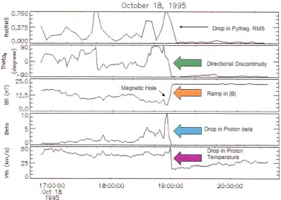
in-volving relatively rapid changes in magnetic field and plasma quantities, and therefore requiring relatively small-scale time averages, appears to be most effective in such front-boundary determination. These depend on the possibility that this boundary has one or more of the following features of suf-ficient size as we enter the MC: (1) a sufsuf-ficiently large di-rectional discontinuity (DD) in the interplanetary magnetic field (IMF), (2) a proton plasma beta (βP)drop, (3) a pro-ton temperature drop, and (4) an increase in the IMF’s inten-sity; see the color arrows in Fig. 1. These criteria were the result of experience gained from many years of visual exam-ination of the profiles of plasma and field quantities around the vicinity of front-side boundaries of numerous MCs (e.g., see Lepping et al., 1990, 2003, 2006; Burlaga et al., 1981; Burlaga, 1995). The first to recognize that a magnetic hole may occur at the front boundary of a MC were Burlaga et al. (1980); and see Burlaga (1995, Fig. 6.10 and related com-ments). See the panel on|B|(3rd down) in Fig. 1 giving an example of a magnetic hole. Hence, we attempted to add to this scheme the search for the existence, and timing, of a pos-sible magnetic hole but found that such structures were not yet sufficiently well characterized quantitatively (nor unique enough) to be reliable in determining a MC’s front boundary. (However, using the existence of a possible magnetic hole as another means of identifying a front boundary is an area that surely could stand further study.) Besides the four cri-teria above, and the existence of magnetic holes, other tests were considered and dismissed as unreliable, insufficiently sensitive, or involving quantities that were too slowly chang-ing for practical use. The early slowchang-ing down of the MC’s internal plasma (due to MC expansion, e.g., see Marubashi, 1997) is one such example of an unreliable test, because the early change in speed near the boundary is usually much too small to be easily detected, even over an hour or so. Changes of the fluctuation level of the IMF (via examination of the root-mean-square deviation (RMS) shown by the top panel of Fig. 1) was also considered with quite unreliable results. In short, incorporating any other than the four criteria listed above did more harm than good in our attempt to estimate the timing of the MC’s front boundary.

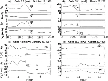
Fig. 1. An example of the profile of a front boundary crossing of a MC, that of 18 October 1995, at approximately hour 19, as seen in WIND field and plasma data. The indicators of the boundary are shown by the color-coded arrows, along with their literal denotations. The quantities plotted are B-RMS (thin black arrow), thetaB(heavy green arrow), magnetic field magnitude,|B|(heavy orange), proton plasma

beta (heavy light blue), andVT h(heavy purple); a magnetic hole, sometimes occurring at a MC’s front boundary, is indicated by a thin

black vertical arrow. Only four of these six quantities (those with heavy colored arrows) will be incorporated into the boundary identification scheme as described in the text, but all six were investigated.

We briefly describe here one of the needs for such a bound-ary estimation program which was suggested above, and that is one to help in forecasting a geomagnetic storm’s mini-mumDst and its timing based on magnetic field and plasma measurements acquired during the passage of the causal MC. To do this, a MC parameter fitting program and an accurate estimate of the MC starting time (front boundary time) are needed in real time. The program starts with a module that encompasses two phases: one for automatically identifying a candidate MC (see, e.g., Lepping et al., 2005; Feng et al., 2007) which is also expected to be able to estimate the MC’s front boundary time (where the preliminary estimate is called

tB)to within at least±2 h of the actual boundary-time, and a second part that produces a refined boundary-time (tB*) using the four criteria, as listed above. Such a forecasting scheme (or any similar one) should be applicable to a large range of MC types but is best applied to North→South types, and starting in the year 2005 such types started to become prevalent, as was suggested by Bothmer and Rust (1997); also see Lepping et al. (2005), Huttunen et al. (2005), Lynch et al. (2005). In particular, we will obtain, through the use of a refined version of a well known MC parameter-fitting

2 Criteria used to obtain an accurate MC front bound-ary time,tB*

Application of the automated MC identification program (Lepping et al., 2005) provides an approximate MC front boundary time, tB. Our attempt now is to use short-scale averages, <t >(5, 10, 15, and 20 min were used), initially based on 1-min averages of the interplanetary magnetic field and 1.5-min averages of plasma quantities, in order to find the more accurate front boundary time, tB*, in the vicinity of the approximatetB-time by searching for possible occurrences of the four key boundary signatures listed in the Introduction and whose formulation is given in detail below. Obviously some of these four signatures may indicate the occurrence of many other interplanetary structures (e.g., abrupt|B|increases could be fast shocks, etc.) besides MCs. But since we examine only in the close vicinity oftB, which we assume must be close to the MC’s actual front boundary, we are almost assured that such major competing signatures will not be confused with an actual MC boundary. The four possible signatures will be examined in the order shown, in the four criteria below. (Note that for each test an entity is calculated every<t >min until a full set is developed over the full range (tB–2 h) to (tB+2 h), and then examined for some outstanding change.)

Test no.

1. DD: Defining an angle change1λ

[=cos−1(<B1>•<B2>/|<B1>||<B2>|) in the mag-netic field, where <B1> (<B2>) is the upstream (downstream) average of the field over <t >, allow-ing a<t >-length transition between], then1λmust be greater than a limit, denoted by1λLto raise a flag. 2. βP drop: Defining

1βP≡(βP1−βP2), where<βP1>(<βP2>)is the up-stream (downup-stream) average ofβP over<t >, allowing for a<t >-length transition between, then1βP must be greater than the limit1βP ,Lto raise a flag.

3. 1TP drop: Defining

RT≡Rel1TP≡1TP/<TP>=2(TP1−TP2)/(TP1+TP2), where<TP1>(<TP2>)is the upstream (downstream) average of proton temperature over <t >, allowing a <t >-length transition between, then RT must be greater than the limit RTLto raise a flag.

4. Marked|B|increase: Defining

R|B|≡Rel1|B|≡2(|B2|−|B1|)/(|B2|+|B1|), where

<|B1|> (<|B2|>) is the upstream (downstream) average of field magnitude over <t >, allowing for a

<t >-length transition between, then Rel, B must be greater than the limitR|B|_Lto raise a flag.

The four limits1λL,1βP ,L, RTL, andR|B|Lwill be deter-mined through optimization below. Different<t >-lengths

will lead to different limit-values. Finally, we examine to see if the “side” of the estimated boundary has a MC-like value ofβP. Specifically we demand thatβP<0.2 or the preliminary estimate is ignored; the value of 0.2 was found through trial-and-error, not through optimization.

For example purposes, Fig. 1 shows the profile of the MC of 18 October 1995 in terms of B-RMS, the latitude of the magnetic field (θB)in GSE coordinates, magnetic field mag-nitude (|B|), proton plasma beta (βP), and thermal speed (VT h), in the panels from top to bottom. Indicated in the figure by four color-coded heavy arrows are the features rel-evant to the specific criteria (above) that are to be tested. (As mentioned in the Introduction, RMS and magnetic holes, also show in Fig. 1, were examined but not used in the scheme.) We now carefully examine the results of apply-ing these four criteria quantitatively to the WIND magnetic field and plasma data (see Lepping et al., 1995; Ogilvie et al., 1995, respectively), by setting up an optimization-function (M) that we call, in order to “optimize” the criteria associ-ated limit-values. Getting the optimum limit-values will re-quire using the optimization-function for each test separately in a statistical manner. Once optimum limit-values are found as applied to a previously known and carefully chosen subset of MCs, i.e., those discovered through inspection of WIND data, we apply these four criteria with the optimum limit-values to a much larger set of MCs, to further test them for finding front boundaries.

3 Developing the scheme

3.1 Data sets used in developing the scheme

The scheme will be applied to three sets of WIND data: (i) to a specially chosen subset (N=26, Set #1) of the combined N6S, S6N MCs (see Tables 1, 3, and 4 of Lepping et al., 2006) with poor quality cases (i.e.,QO=3 cases) deleted (see Appendix A of Lepping et al., 2006, which defines quality,

QO), (ii) to the (N0=122, Set #2) MCL events found by Lep-ping et al. (2005), and (iii) to the set (N00=81, Set #3) of MCs in Lepping et al. (2006) which includes all MCs visually identified in the period from the beginning of the WIND mis-sion in late 1994 to August of 2003. However, the application of the program to Set #3 will be considered to be a final test of the scheme, whereas the use of Set #1 is for determining the limits (fixed numbers) used in the scheme through the op-timization, and use of Sets #1 and #2 together are for deter-mining the best<t >to use and for describing its capabilities and breath of applicability generally. The start-times for the MCL events are listed on a page on the WIND/MFI Website given by http://lepmfi.gsfc.nasa.gov/mfi/MCL1.html.

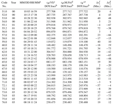
Table 1. MC Front Boundary Times (tB(VI)) Chosen by Visual Inspection, by the Model Fitting routine, and by the Boundary Estimation

Scheme (tB*) for WINDN=81 WIND cases.

Code Year MM/DD/HH/MMa tB(VI)c tB(M.Fit)d tB*e 1t₁f 1t₂g

No. DOY.fractb DOY.fractb DOY.fractb (Min.) (Min.)

1.0 95 02 08 05 41 039.237 039.242 039.255 25 6

2.0 95 03 04 11 40 063.487 063.450 063.500 19 −53

2.2 95 04 03 07 43 093.322 093.325 093.330 12 5

3.0 95 04 06 07 21 096.306 096.304 096.307 1 −3

4.0 95 05 13 10 25 133.434 133.454 133.437 4 29

5.0 95 08 22 21 55 234.914 234.887 234.932 26 −38

6.0 95 10 18 19 01 291.793 291.825 291.814 31 47

7.0 95 12 16 04 49 350.201 350.221 350.223 31 28

8.0 96 05 27 14 45 148.615 148.637 148.631 24 33

9.0 96 07 01 17 27 183.727 183.721 183.750 33 −9

10.0 96 08 07 11 56 220.498 220.512 220.457 −59 21

11.0 96 12 24 03 03 359.127 359.117 359.121 −9 −15

12.0 97 01 10 04 58 010.208 010.221 010.238 44 19

13.0 97 02 10 02 43 041.113 041.142 041.124 15 41

14.1 97 04 11 05 53 101.246 101.233 101.325 114 −18

14.2 97 04 21 14 15 111.594 111.604 111.627 48 15

15.0 97 05 15 09 50 135.410 135.379 135.400 −15 −45

16.0 97 05 16 06 39 136.277 136.254 136.299 32 −33

17.0 97 06 09 01 22 160.057 160.096 160.068 16 56

18.0 97 06 19 05 37 170.235 170.212 170.224 −15 −32

19.0 97 07 15 09 07 196.380 196.367 196.402 32 −19

20.0 97 08 03 13 51 215.577 215.587 215.595 26 15

21.0 97 09 18 00 31 261.022 261.021 261.055 47 −2

22.0 97 09 22 01 31 265.064 265.033 265.073 13 −44

23.0 97 10 01 17 07 274.714 274.679 274.723 13 −50

24.0 97 10 10 22 07 283.922 283.992 283.898 −34 101

25.0 97 11 07 15 37 311.651 311.658 311.660 13 11

26.0 97 11 08 05 51 312.244 312.204 312.249 8 −57

27.0 97 11 22 15 09 326.631 326.658 326.665 49 39

28.0 98 01 07 02 55 007.122 007.137 007.135 19 23

29.0 98 01 08 15 55 008.663 008.621 008.702 56 −61

30.0 98 02 04 04 51 035.202 035.188 035.209 10 −21

31.0 98 03 04 14 40 063.612 063.596 063.618 9 −23

32.0 98 05 02 12 52 122.537 122.512 122.559 32 −35

33.0 98 06 02 10 30 153.438 153.442 153.438 1 6

34.0 98 06 24 16 30 175.688 175.700 175.722 50 18

35.0 98 08 20 11 27 232.477 232.429 232.539 89 −69

36.0 98 09 25 10 37 268.443 268.429 268.506 91 −19

37.0 98 10 19 04 22 292.182 292.212 292.199 24 44

38.0 98 11 09 00 07 313.005 312.992 313.023 26 −19

39.0 99 02 18 12 22 049.515 049.596 049.549 48 116

41.0 99 08 09 10 19 221.430 221.450 221.439 13 29

42.0 99 09 21 20 27 264.852 264.879 264.845 −10 39

43.0 00 02 12 17 31 043.730 043.713 043.774 63 −26

44.1 00 02 21 10 15 052.427 052.408 052.410 -25 −27

44.2 00 06 24 07 37 176.318 176.346 176.342 35 40

44.3 00 07 01 08 48 183.367 183.367 183.329 −54 0

45.0 00 07 15 07 05 197.296 197.283 197.364 98 −18

46.0 00 07 15 19 55 197.830 197.879 197.865 50 70

47.0 00 07 28 20 13 210.843 210.879 210.880 53 52

48.0 00 07 31 23 30 7213.979 214.004 213.990 16 36

49.0 00 08 12 06 22 225.265 225.254 225.304 56 −16

Table 1. Continued.

Code Year MM/DD/HH/MMa tB(VI)c tB(M.Fit)d tB*e 1t₁f 1t₂g

No. DOY.fractb DOY.fractb DOY.fractb (Min.) (Min.)

51.0 00 10 03 16 59 277.708 277.712 277.722 20 6

52.0 00 10 13 17 38 287.735 287.767 287.738 4 45

53.0 00 10 28 22 30 302.938 302.971 302.965 40 48

54.0 00 11 06 22 44 311.948 311.962 311.950 3 21

55.1 01 03 20 00 25 079.018 078.971 079.015 −4 −67

55.2 01 03 20 18 25 079.768 079.742 079.818 72 −38

56.0 01 04 04 20 52 094.870 094.871 094.872 3 1

57.0 01 04 12 09 00 102.375 102.329 102.391 23 −66

58.0 01 04 22 01 08 112.048 112.037 112.036 −17 −15

59.0 01 04 29 01 43 119.072 119.079 119.100 40 10

60.0 01 05 28 11 34 148.482 148.496 148.470 −18 19

61.0 01 07 10 18 31 191.772 191.721 191.795 34 −73

62.0 01 10 31 22 00 304.917 304.888 304.930 19 −42

63.0 01 11 24 16 52 328.703 328.658 328.713 14 −65

64.0 02 03 19 23 42 078.988 078.954 078.959 −41 −48

65.0 02 03 24 03 17 083.137 083.158 083.151 19 30

66.0 02 04 18 04 37 108.193 108.179 108.194 2 −20

67.0 02 04 20 12 00 110.500 110.492 110.576 109 −12

68.0 02 05 19 03 22 139.140 139.163 139.157 24 32

69.0 02 05 23 23 58 143.999 143.975 143.983 −23 −35

70.0 02 08 01 11 43 213.488 213.496 213.518 43 11

71.0 02 08 02 07 15 214.302 214.308 214.300 −3 9

72.1 02 09 03 00 22 246.015 246.012 245.976 −57 −4

72.2 02 09 30 21 57 273.915 273.942 273.909 −8 39

73.0 03 03 20 12 36 079.525 079.496 079.547 32 −42

74.0 03 06 17 19 01 168.792 168.742 168.804 17 −73

75.0 03 07 10 20 33 191.856 191.829 191.875 27 −39

76.0 03 08 18 11 24 230.475 230.483 230.488 19 12

a_{MM/DD/HH/MM refers to month (MM), day-of-month (DD), hour (HH), and minute (MM) for the visual inspection time.} b_{DOY.fract. means day of year and fraction of day-of-year.}

c_t

B(VI) is the front boundary-time derived from visual inspection of the data in DOY.fract. d_t

B(M.Fit) means the front boundary-time used in the Model Fitting in DOY.fract. e_t

B* is the “refined” time, in DOY.fract, estimated by the front-boundary estimation program developed here. f_1t

1is defined as [tB*–tB(VI)]; these values have a minimum uncertainty of±2.5 Min but it is always somewhat larger depending on how

many specific tests were passed for any given event and their spread oftB*-estimates. g_1t

2is defined as [tB(M.Fit)–tB(VI)]; these values have a minimum uncertainty of±1 Min but it is always considerably larger depending

on various factors, especially on the kind of average used in the MC fitting, usually being one of 15 Min, 30 Min, or 1 h averages.

that each event is coded (K) from 1 to 99, even though there are 106 initial events, because there are some “inserted” events that are essentially subscripted, e.g., MCs with num-bers 2.2, 14.1, 14.2, 44.1, etc.

3.2 Statistical optimization of the limit-values: founda-tion

The optimization function, for a specific set of test MCs, will depend on two features: (1) it takes into consideration the number of events that passed and (2) it measures how well the events passed these tests, meaning an examination is made of a given criterion’s ability to accurately reproduce a

previously and carefully determined start-time through visual inspection (VI), i.e., in terms of

Once our scheme determines the optimum limit-values (using Set #1), and the proper averages to use, they are then fixed in the scheme for all future use. Now1t1is defined as the difference in time betweentB(VI) and the time estimated by the our scheme for each event, calledtB* when applied to any future data set of actual MCs (not just a test-set) and in particular on Set #3; hence,

1t1= [tB∗−tB(VI)], (2) As in the case of1t, 1t1 is based on an average value of

tB* for each MC and therefore, 1t1 is an average. Sim-ilarly, and only for completeness, we define another time-difference, i.e.,

1t2= [tB(M.Fit)−tB(VI)], (3) wheretB(M.Fit) is the time listed for the front boundary as was used in MC fitting. In Table 1 three estimated front boundary times are given [tB(VI),tB*, andtB(M.Fit)], and the two difference-times given by Eqs. (2) and (3), for the full N=81 WIND MC cases, where each MC carries the same code number K (first col.) as was used in the Web-site listed above, as of 1 April 2008. The timestB(VI) in the Table 1 will be used in any comparison to the automati-cally determined boundary-time by our scheme for an actual MC, whether it be from data Set #1 or Set #3. (Notice that thetB(VI) time is given in two formats in Table 1 for con-venience; see footnotes a, b, and c for the table.) The time

tB(VI) usually differs (i.e., by 1t2)from any front bound-ary times that we have given earlier for these 81 MCs, when MC parameter-fitting was considered. (This is the reason for showing the1t2’s in Table 1; they are not used directly in this boundary analyses.) This is so, because in carrying out the MC fitting, using Lepping et al. (1990) we often had to make some front boundary adjustments (based on the fit of data all across the full MC), especially if the cloud was very asymmetric. Usually this was of little consequence in the outcome of the fitting, since relatively large averages were often used in the fitting, viz, 15, 30, or 60 min. However, if our MC fitting model had taken into account the MC’s inter-action with the upstream plasma, and MC expansion, there would likely be a significantly smaller average difference of

1t2.

3.3 Limit-value determinations from the Magnetic Cloud front boundary tests: concepts

From previous work and inspection of magnetic clouds the test-limits are known to exist somewhere in the range of:

Test 1 : 1◦≤limit≤99◦

Test 2, 3, and 4 : 0.01≤limit≤0.99

The range in test #1 is searched in 1 degree intervals. The ranges in tests 2, 3, and 4 are searched in 0.01 intervals. For each limit-value theN=26 combined N→S and S→N events of Set #1 (as described above) are tested as a set (within the±2 h interval around the visual inspection time, or±2 h

around an automatically determined time for Set #2, for ex-ample), and the values for the two following quantities are calculated:

– The fraction of events passing the test (“feature 1”) – The average error in the estimate of the boundary time

(“feature 2”)

These quantities are then used to maximize the “optimization-function” (M) (specifically defined be-low), in order to determine the “best-choice” limit-value for a given type of average,<t >, for each test. In turn, M is applied to each of the four averages (5, 10, 15, 20 min) separately. Specifically the maximization is carried out on this optimization function:

M(limit-value)=(0.5×fraction of events passing) +(1− |(average error/120.)|) (4) The form of M is chosen to place more weight on the av-erage error at each trial, compared to percentage passing a given test. The idea is that there are four independent tests to find the front boundary time for each MC, so for any given test the average error is weighted more than the fraction of events passing that test. Note that average error is measured in minutes and 120 (minutes) is the total possible error, so the average error is divided by 120 to get a fraction of the total error. Hence, both terms are expressed as fractions. The maximum possible value ofM is therefore 1.5, where then the fraction passing would be 1.0 and the average error would be 0.0. The optimum limit for each test is then found when

M is maximum. Specifically this is done by starting with test #1, and for a given type of average (say 5 min), going through all of the MCs of a given set at a fixed trial limit, re-peating this for another slightly larger limit, etc. until a set of Ms is derived from which we choose the maximum one and its associated limit. This then is the optimum limit for that test. This is repeated for test #2, test #3, and test #4. Then the whole procedure is repeated for a different type of aver-age (say 10 min now), etc., until we derive the limit-values associated with the set of max Ms for all four types of aver-ages, for a given data set. Finally, in order to rule out “false positives” (e.g., say only one event passed and with small er-ror yielding a misleadingly large value of M), we added a new condition that the fraction of events passing a given cri-teria (feature 1) must be at least 0.25 or else the limit-value is discarded.

3.4 Application to data sets #1 and #2 to find test-limits and optimum average

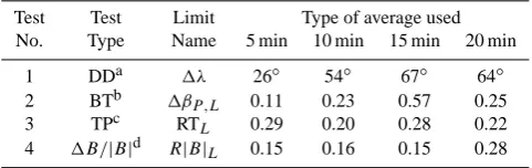
Table 2. Criteria limit-values found through M-function optimiza-tion.

Test Test Limit Type of average used No. Type Name 5 min 10 min 15 min 20 min

1 DDa 1λ 26◦ 54◦ 67◦ 64◦

2 BTb 1βP ,L 0.11 0.23 0.57 0.25

3 TPc RTL 0.29 0.20 0.28 0.22

4 1B/|B|d R|B|_L 0.15 0.16 0.15 0.28

a_{Directional discontinuity (DD) in the IMF} b_{Proton plasma beta}

c_{Relative proton temperature difference}

d_{Relative interplanetary magnetic field (IMF) intensity difference}

the test-limit-values in Table 2. However, below in apply-ing the scheme to both Data Sets #1 and #2, we attempt to find which type of average is optimum for application of the boundary scheme at 1 AU. Figures 2 through 7 show various histograms of relevant quantities, presented to aid in find-ing that optimum limit-set and optimum average, and fur-ther to give some measure of the strengths and limitations of the overall scheme. Strictly speaking, when finding the limits Eq. (1) holds only when using actual MCs where vi-sual inspection was possible, e.g., Set #1. (This is true also of Set #3, but limit testing is not done for that set.) When data Set #2 is used, we are applying an equation that is very similar to, but not exactly the same as, Eq. (2), i.e., now

1t0= [t_B∗(test)−tB(auto)], (5) wheretB(auto) is that estimated front boundary-time found from the MC auto-identification program (see Lepping et al., 2005), replacing the visually inspected time. (Again, a given1t0 is a single number for a given MCL event based on an average of time-differences from the four possible cri-teria.) This is important, because then we wish to find the difference in boundary identification times (1t0s) between two automatic identification/estimation programs, i.e, MC-identification program (Lepping et al., 2005) and boundary-identification program, sequentially. After all, in a predic-tion/forecasting scheme there would be no visual inspection option available. The1t’s (from Set #1) and the1t1’s (from Set #3) are properly considered errors (if the VI’s are well estimated, a fair assumption), but the1t0’s are not strictly errors, because we cannot be sure that the front boundary times of the automatically identified MCL events are more accurately chosen than the times from this scheme.

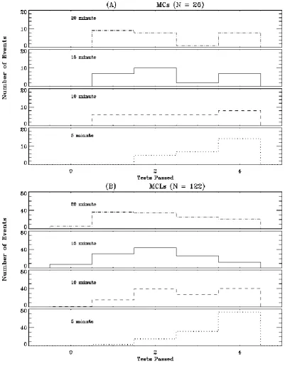
Figure 2a, b shows histograms of the number of WIND MC events that passed a given number of tests, up to the maximum of four tests for the various averages 5, 10, 15 and 20 min separately. In Fig. 2a the results for the MC Set #1 are shown, where theN=26 specially chosen MCs are used. No-tice that, for the 5 min tests, all events occur in the last three

bars. So there was not a single MC that did not obtain at least two time-estimates from the tests. Also, the 5-min dis-tribution is such that the frequence of occurrence grows with the greater number of test passed, in contrast to the other averages. From the point of view of Fig. 2a the 5 min av-erage cases gave the best results among the four different types of averages. Figure 2b is for the MCL Set #2 with

N=122 events. Similar to Fig. 2a, almost all cases fall into the last three bars. And the situation is generally the same as in Fig. 2a, where the frequence of occurrence grows with the greater number of test passed, etc. Again, from the point of view of 2B the 5 min average cases were the best results among the four different types of averages.

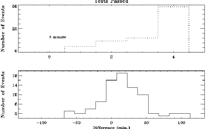
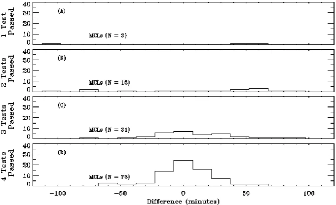
Figure 3a, b shows histograms giving the number of WIND MCs that fall into time-differential buckets, where the time difference (1t) for any one case is defined by Eq. (1). Notice that with this sign-choice of 1t, all resulting 1t -values such as those given in Fig. 3a, b, will have the MC part on the right of the zero-point in time, and the upstream region (usually a sheath region) on the left of the zero-point. The histogram of Fig. 3a applies to data Set #1’sN=26 MCs. Notice that the 5 min tests in Fig. 3a (fourth panel down) provide the best overall results, in the sense that their his-togram best approximates a normal distribution, has fewest “outliers,” and peaks around zero. Notice that for the 5 min averages all but one event of the 26 total events occur within

±50 min, and there are 20 MCs (i.e., 78%) that occur within

±30 min. The histogram of Fig. 3b is similar to Fig. 3a ex-cept it applies to theN=122 MCL events (Set #2), and again the 5 min tests provide the best overall results, although its case is somewhat weaker, since more events occur outside

±50 min. We can say, however, that of all of the histograms in Fig. 3b, the histogram for the 5 min averages is most sym-metric about zero, there are few outliers in the negative range (probably strongest argument for this average), and it has fewest extreme cases (i.e., >50 min) in the positive range. Notice that within±50 min there are 108 MCs, which is 89% of the fullN=122 MCL events, and within ±30 min there are 97 MCLs (i.e., 80%). One final point to be made about Fig. 3b, for the 5 min panel, is that there is greater symmetry compared to that panel of Fig. 3a; this is probably due to the poorer statistics of Fig. 3a.

From overall considerations of Fig. 2a, b and Fig. 3a, b, we determine that the 5 min average tests are generally the most optimum with respect to both the shape of the related occurrence distributions and the distributions of the associ-ated1tvalues. Hence, we will assume that these are general findings (for at least 1 AU) and display future figures only for the 5 min average tests.

Fig. 2. (A) Histograms showing the number of WIND MC events that passed a given number of tests, up to a maximum of four tests, for the

N=26 specially chosen MCs – see text (Data Set #1) with no regard to the specific nature of the test (i.e., test no.). From top to bottom, the dashed-dot histogram is for the 20 min average study; the solid-line histogram is for the 15 min average study; the dashed-line histogram is for the 10 min study; and the dotted-line histogram is for the 5 min study. (B) Similar to (A) except the histograms apply to the N=122 MCL event set (Data Set #2).

there were no events that fell into one test passed. For ex-ample, Fig. 2a reveals that 7 events passed three tests, and Fig. 4b shows the specific 1t’s that were associated with those seven-passed-test cases. Likewise, panel (4C) shows

Fig. 3. (A) Histograms giving the number of WIND MCs (Data Set #1) that fall into time-differential buckets, where Difference refers to1t=[tB*(test)–tB(VI)]. The scheme for the display of type of averages is the same as used in Fig. 2a, b. (B) Similar to (A) except the

histograms apply to theN=122 MCL (Data Set #2) events and Difference refers to1t0=[tB*(test)–tB(auto)].

case exceeded a1tof 50 min (and not surprising, it had only one-test-passed), and most1ts were well under 30 min.

Figure 5 shows histograms of1t0s, similar to those shown in Fig. 4, but now for the 122 MCL events of data Set #2, that passed a given number of tests, up to the full

Fig. 4. Histograms of1t=[t_B*(test)–t_B(VI)] for theN=26 MCs of Data Set #1 that passed a given number of tests, up to the full number of four tests for the 5 min averages. We know from Fig. 2a that no events occurred in either the “zero tests passed” or the “one-test passed” categories. But 5 events passed the two-test category and their1t’s are shown here in (A). (B) Shows the specific 71t’s that were associated with the three-tests-passed case. Likewise, (C) here gives the distribution of1t’s for the 15 events that passed all four tests.

Fig. 5. Histograms of1t0=[tB*(test)–tB(auto)], similar to those shown in Fig. 4, but now for the number ofN(total)=122 MCLs of Data

Set #2 that passed a given number of tests, up to the full number of four, for the 5 min averages. For example, Fig. 2b reveals that 15 events passed two tests, and (B) here shows the 15 specific1t0’s that were associated with those 15 cases. Likewise, Fig. 2b reveals that 17 events passed four tests, and (D) here gives the distribution of the specific1t’s for the 17 events that passed all four tests, etc.

shows the distribution of1t0’s for the 31 events that passed three tests that were indicated in Fig. 2b, etc. It is clear that the1t0-distributions of Fig. 5c, d are more symmetric about

1t0=0.0 and better peaked than those in the other two panels. Also, Fig. 5 shows quite a few cases where|1t0|of 50 min is exceeded, unlike the situation of Fig. 4. However, Fig. 5c, d are quite acceptable which argues for the obvious importance of having a large number of tests passed.

Fig. 6. Histograms giving the number of MCs that contributed to the estimate of a given1ti=[tB*(test)i–tB(VI)] (i=1,.., 4), individually for

the following: test #1 (A, DD), test #2 (B,1βP), test #3 (C,1Temp.), and test #4 (D,1|B|), for the N(total) = 26 MCs of Data Set #1,

based on the 5 min averages. The subscripts in the1ti-equation here mean that the1t’s for every individual test’s estimate are being shown,

not just the average1t, so this differs from Eq. (1).

Fig. 7. Histograms giving the number of MCLs that contributed to the estimate of a given1t_i0=[tB*i–tB(auto)], individually for the following:

test #1 through test #4, according to the same scheme as in Fig. 6, but now for theN(total)=122 MCLs of Data Set #2, based on the 5 min averages. The subscripts in the1t_i0-equation here mean that the1t0’s for every individual test’s estimate are being shown, not just the average1t0.

were relatively symmetric, centered at or near the Difference of 0.0, and had fewer that occurred far from 0.0, although the Ns for both of these were slightly lower than for tests #1 (Fig. 6a) and #3 (Fig. 6c), which were spread over a much greater range, especially into the sheath region. Only test #1 (Fig. 6a) gave any distant positive estimates (actually only one), near 100 min.

3 4 5 6

Hour Hour

10 11 12 13

(c) Code 12.0 (n=4) January 10, 1997 (d) Code 56.0 (n=2) August 20, 1998

18.0 18.5 19.0 19.5 20.0 0 0.25 0.50 0.75 1.0

(a) Code 6.0 (n=4) October 18, 1995 (b) Code 55.1 (n=2) March 20, 2001

10 60 35 0.0 0.5 10 0 20 1.0 -900 90 0 25 500 3 6 30 15 0 90 0 -90 Vth (km/s) βP B (nT) θB βP θB B (nT) Vth (km/s) 10 35 60 0.0 0.50 10 20 -90 -90 0 -90 -90 0 10 1520 25 0.0 0.110 15

*

*

*

*

*

*

*

*

*

*

*

*

*

*

*

*

Fig. 8. Four examples of profiles of the quantities used in identifying a MC’s front boundary, for±3 h around an earlier-determined VI boundary time (shown by a vertical dashed line). The quantities plotted are the field direction,θB (test #1), field magnitude,|B|(test #2),

proton plasmaβP (test #3), and thermal speed,VT h(test #4). These MCs are: (A) DOY 291 (18 October), 1995; (B) DOY 079 (20 March),

2001; (C) DOY 010 (10 January), 1997; and (D) DOY 232 (20 August), 1998. The estimated boundary times are given by the front edge of the symbols (in the panels from top to bottom): DD (time of directional discontinuity), dB (del-field magnitude), BT (proton plasma beta), PT (proton temperature, in terms of thermal speed). Then’s represent the number of tests passed for each case. From the individual tests a net estimate is obtained, called here thet_B*-time, which is also shown as the symbol*. We can see the difference in time between the vertical dashed line (the VI time) and thetB*-time, given as1t1, in each case. See Sect. 3.3 for a definitions of the VI time and1t1(Eq. 2). The

“Codes” are explained in the text.

were only slightly asymmetric with respect 0.0, but distri-butions (A) and (C) were significantly asymmetric. Fortu-nately many cases passed, but the1|B|test (panel d) was a rather weak contributor with onlyN=82. The best type of test for the MCLs was theβP test, with the best symmetry, few events in the sheath, and a strong peak, and the poorest type of test was a tossup between the DD test (A) and the Temp. test (D). Even with all of the asymmetries seen in the panels of Fig. 7 when put together the result is only slightly asymmetric, as seen in Fig. 3b for the 5 min panel.

Figure 8 shows four examples of profiles of the physical quantities used in identifying a MC’s front boundary, where from top left to bottom right are for the MCs of (A) 18 Oc-tober 1995 (an excellent case), (B)20 March 2002 (a good case), (C) 10 January 1997 (a fair case), and (D) 20 August 1998 (a poor case). The quantities plotted are field direction,

θB (for test #1); field magnitude, |B| (for test #4); proton plasmaβP (for test #2); and thermal speed,VT h(for test #3). The center of the symbols (DD, dB, etc.) give independent

Fig. 9. Histograms considering theN=81 WIND MC set (Data Set #3) for the period early 1995 to August 2003, for the 5-min tests only. (Top) Histogram showing the number of MC events that passed a given number of tests, up to a maximum of four tests with no regard to the specific nature of the test. (Bottom) Histograms giving the number of MCs that fall into time-differential buckets, where the time difference now is1t1=[tB*–tB(VI)].

±one standard deviation of those four. Then that final aver-age was determined to be tB*. However, for the overall set of 81 MCs (Set #3, as we will discuss below) the final results were not as good as simply taking a straight average. Hence, we eliminated this editing routine.)

It has been shown that for bona fide MCs (with relatively strong |B|, long durations, and relatively good flux rope structure), as well as for the usually less impressive (i.e., ac-cording to strength of|B|and flux rope structure) MCLs by the same standards, 5 min averages are the best to use in the four tests defined in Sect. 2. We should stress, however, that it was apparent from these and results not shown that the re-sults of the scheme do not depend crucially on the 5 min aver-age; e.g., the 10 min averages may have done almost as well, the 15 min averages also appeared acceptable if borderline, but the 20 min averages would clearly not be acceptable.

4 Tests of scheme using the full set #3 of WIND MCs Figure 9 shows two histograms that give the results of the ap-plication of the boundary scheme for the “full” WIND MC set for the first 8.6 years of the mission for the test-limits associated with the 5-min averages. Hence, results from all three quality levels,Q=1,2,3 of the originalNT=82 WIND MCs were initially incorporated in this part of the study. We point out, however, that one MC was dropped, because of the inaccessibility of needed plasma data for some tests at the time of this study. Hence, the resulting data set (Data Set #3) is based onN=81 MCs. Figure 9 (top) is a histogram

Fig. 10. Histograms giving the number of MCs that contributed to the estimate of a given1t1i=[tB*i–tB(VI)] (i=1, ..., 4), individually for

the following: test #1 (A, DD test), test #2 (B,1βP), test #3 (C,1Temp.), and test #4 (D,1|B|)for theN(total)=81 MCs of Data Set #3,

based on the 5 min averages. The subscripts in the1t1i-equation here mean that the1t1’s for every individual test’s estimate are being

shown, not just the average1t1.

Figure 9 (bottom) shows a histogram that gives the number of MCs that fall into time-differential buckets, where the time difference is now equal to1t1. This1t1-distribution gives a good measure statistically of the accuracies of the scheme’s estimates of the front boundary-times, being limited only by the accuracy with which these times were estimated by vi-sual inspection (VI) in the first place. But we should keep in mind that the time-estimation from visual inspection may it-self be inaccurate in a few complex cases. Figure 9 (bottom) indicates that 591t1s (i.e., 73% of the full 81) lie within

±30 min, 711t1s (i.e., 88%) lie within±45 min, and only 5 cases lie outside a|1t1|of 1.0 h, which is only 6% of the full set, and these 6% would be considered unsatisfactory. Since MC parameter fitting is usually done on the basis of 30 or 60 min averages on MCs that are typically 20 or so hours in duration, these results seem quite satisfactory generally.

Figure 10 shows histograms giving the number of the 81 MCs that contributed to the estimate of a given1t1i, (i=1, ..., 4) specifically for test #1 (Fig. 10a), test #2 (Fig. 10b), etc., for data Set #3. As we see, there were 77, 60, 74, and 56 tests, respectively, that passed, summing to 267 (or 82%) of a possible max of 324 (=4 tests×81 MCs). Clearly tests # 2 (Fig. 10b, test onβP)and #4 (Fig. 10d, test on1|B|)give the best results in that the distributions were relatively symmet-ric, centered near a1t of 0.0, and they had fewer cases that occurred beyond|1t1|of 45 min. However, the Ns for both of these are slightly lower than for tests #1 (Fig. 10a) and #3 (Fig. 10c), which are spread over a much greater range, es-pecially into the sheath region. Clearly there were few cases of|1t1i|beyond 45 min for three of the tests; theTP-test (B) was an exception. It is evident that the TP-test is the

poor-Abs. Value of Diff. (min.)

1

0

4

3

2

0

120

100

80

60

40

20

MCLs and MCs (N = 203)

Test Passed

Fig. 11. The absolute value of either1t1=[tB*–tB(VI)] (for the

MCs) or1t₁0=[tB*–tB(auto)] (for the MCLs) is plotted against the

number of tests passed for the combined results of all 81 MCs (black crosses) and 122 MCLs (red triangles). In each column, i.e., for each fixed number of tests passed, we indicate by a small black box where the average value is located, and we connect the boxes with line segments to emphasize the trend, which clearly shows smaller differences for greater number of tests passed.

est, and this was also true for Set #1. This fact aboutTP is interesting, since theβP test is so good for all data sets, and it is strongly dependent on proton temperature (as well as on density and IMF intensity).

5 Summary and discussion

criteria, and it was extensively tested using WIND magnetic field and plasma data for specific MCs and MC-like events (MCLs). The program for implementing this scheme is at the Website: http://wind.nasa.gov/mc/boundary.php. The four criteria used in the scheme involved examining the magnetic field and plasma data for generally well known MC front-boundary indicators, such as field directional change, proton plasma beta drop, proton temperature drop, and moderately strong positive gradient in the field magnitude as the MC is entered. Other criteria were tested, such as an examination of a normalized (by|B|)drop in RMS of the field, beginning of a drop in the plasma speed (as would be expected for an expanding MC), as well as evidence of a magnetic hole, and they all were found to be unreliable and generally not use-ful. A specially chosen subset ofN=26 MCs (Data Set #1) of the first 81 MCs discovered in the WIND data set over the mission’s first 8.6 years were used to optimize the limit-values in the four criteria used in finding the boundaries, as defined in Sect. 2. By this we mean that all empirically de-termined parameters were found through the use of this data via the maximization of a so-called “optimization function” (M); see Eq. (4). Table 2 provides the resulting limit-values for the four criteria. Data Set #1 plus the MCLs (Data Set #2) ofN0=122, found from an auto-identification program (Lep-ping et al., 2005) from this same overall WIND data were used to determine what kind of average of the data was op-timum for use in the scheme; 5 min averages were found to be slightly optimum. That is, we determined that generally using 5 min averages of the field is best for application of this scheme at 1 AU, but the scheme’s success was not crucially dependent on the type of average used; 10, 15, and 20 min averages were also considered with 10 min averages giving almost the same level of success.

Final testing of the first 81 WIND MCs (Data Set #3), which followed from application of the four tests described above using the derived limit-values of Table 2 and 5 min averages, showed that 73% of the1t1s lie within±30 min, 88% lie within±45 min, and only 6% lie outside a|1t1|of 1.0 h, and only these 6% would be considered unsatisfactory. Since MC parameter fitting is usually done on the basis of 30 or 60 min averages, these results generally seem satisfac-tory, at least by that standard. This relatively large set of 81 MCs covers various types, sizes, internal field intensi-ties, and axial attitudes, so they are a broad representation of MCs at 1 AU. Hence, the success rate of 75 out of 81 MCs (i.e., 93%), which had 2 or more tests used in estimating the boundary, as seen in Fig. 9 (top), suggests that for about 90% of the time this scheme should be successful for MCs at 1 AU generally. Notice that this percentage agrees with the figure of 88% of the cases lying within±45 min, although this does not suggest that they are the same MCs.

By combining the results of all|1t1|=|tB*−tB(VI)| for the MCs and all for all|1t0|=|tB*−tB(auto)|for the MCLs (givingNT=203 events) and plotting the absolute value of ei-ther the|1t1|s or the|1t0|s against the number of tests passed

we obtain Fig. 11; black crosses are used for the MCs and red triangles for the MCLs. (For convenience we will call “Diff” either a|1t1|or a|1t0|here.) In this figure we indicate by a small black box where the average value of the combined crosses and triangles (the Diff’s) is for each column, i.e., for each fixed number of tests passed, and we connect the boxes by straight lines. It is apparent that there is a statistical de-pendence of accuracy of the estimate of boundary time on the number of tests passed, whereby the more tests passed the closer the black box is to Diff=0.0, as would be expected. But obviously the dependence is rather weak beyond one test passed. The statistics on column one of Fig. 11 is especially poor since there is such a big spread of values of Diff, and they appear to cluster roughly in two parts, somewhat above and below the black box. We also point out that the spread of Diff values decreases as the number of tests-passed grows, also as expected.

Ivanov et al. (2003) examine various features of one of our MCs, that of 15 May 1997 (Code number 15 in our Ta-ble 1). They discuss many more MC features than we do; our interests are with estimating only the front boundary time. But it appears that we are in good agreement on the front boundary estimation time: they give a time of 09:51:15 UT (their Table 2), and we provide a visual inspection (VI) time of 09:50 UT±1 Min (i.e., DOY=135.410) and a scheme esti-mated time oftB*=0936±2.5 Min (i.e., DOY=135.400), giv-ing a1t1=−15 Min; see our Table 1 and footnotes f and g. We stress that we are not able to give more accurate esti-mates than ±2.5 Min for tB*, which is ±0.0017 of a day, but sufficient for our purpose, which is to be able to provide good starting times for the fitting of MCs that are typically 20 h in duration. And we point out that the uncertainty of

±2.5 Min is the minimum uncertainty due only to the limita-tion of the type of averages used. The actual uncertainty is al-ways somewhat larger depending on how many specific tests were passed, for any given event, to find the tB*-estimate and its spread of individual test-estimates. In fact, for the 15 May 1997 case the size of|1t1|itself is indicative of the size of the actual uncertainty ontB*, of course, if we trust thattB(VI) was well chosen. Finally, we notice that Ivanov et al. (2003) do not list the MC of 16 May 1997 in their ta-ble or in their Fig. 8, whereas we list this event as our Code number 16 in Table 1, and it has a VI front boundary time of DOY=136.277.

Our scheme should be useful for determining in real-time an accurate front-boundary time,tB* (i.e., to about±45 min for a large percentage of cases), after a MC has been detected by some automatic identification program, such as that de-veloped by Lepping et al. (2005) (also see Feng et al., 2007), where the front boundary time was usually not known to bet-ter than±2.1 h. This “refined” estimatetB* is based on anal-ysis of a relatively large number of MCs and MCL events. Finally, we point out that this scheme should also be useful in checking for consistency of the MC front-boundary times chosen by visual inspection after MC data are collected on ground. In many cases accurate after-the-fact front bound-aries are needed for reliable correlation analyses of various MC features, such as suprathermal electrons with relative in-ternal MC regions (e.g., Crooker et al., 2008).

Acknowledgements. We thank the WIND/MFI and SWE teams, for

the care they employ in producing the plasma and field data used in part of this work, and in particular we thank Keith Ogilvie, the SWE principal investigator, and Adam Szabo (PI) and Franco Mariani of the MFI team. This work was supported by the NASA Heliophysics Guest Investigator Program under grant numbers NNG08EF51P and NNX07AH85G.

Topical Editor R. Forsyth thanks E. Romashets and another anonymous referee for their help in evaluating this paper.

References

Bothmer, V. and Rust, D. M.: The field configuration of magnetic clouds and the solar cycle, in: Coronal Mass Ejections, Geophys. Monogr. Ser., vol. 99, edited by: Crooker, N., Joselyn, A., and Feynman, J., AGU Washington, D.C., 139–146, 1997.

Burlaga, L. F.: Magnetic clouds: Constant alpha force-free config-urations, J. Geophys. Res., 93, 7217–7224, 1988.

Burlaga, L. F.: Interplanetary Magnetohydrodynamics, Oxford Univ. Press, New York, 89–114, 1995.

Burlaga, L. F., Sittler Jr., E. C., Mariani, F., and Schwenn, R.: Mag-netic loop behind an inter- planetary shock: Voyager, Helios, and IMP-8 observations, J. Geophys. Res., 86, 6673–6684, 1981. Crooker, N. U., Kahler, S. W., Gosling, J. T., and Lepping,

R. P.: Evidence in magnetic clouds for systematic open flux transport on the Sun, J. Geophys. Res., 113(A12), A12107, doi:10.1029/2008JA013628, 2008.

Feng, H. Q., Wu, D. J., and Chao, J. K.: Size and energy distri-butions of interplanetary magnetic flux ropes, J. Geophys. Res., 112, A02102, doi:101029/2006JA011962, 2007.

Gosling, J. T.: Coronal mass ejections and magnetic flux ropes in interplanetary space, in: Physics of Magnetic Flux Ropes, Geo-phys. Monogr. Ser., vol. 58, edited by: Russell, C. T., Priest, E. R., and Lee, L. C., pp. 343–364, AGU, Washington, D.C., 1990. Huttunen, K. E. J., Schwenn, R., Bothmer, V., and Koskinen, H. E. J.: Properties and geoeffectiveness of magnetic clouds in the rising, maximum and early declining phases of solar cycle 23, Ann. Geophys., 23, 625–641, 2005,

http://www.ann-geophys.net/23/625/2005/.

Ivanov, K. G., Belov, A. V., Kharshiladze, A. F., Romashets, E. P., Bothmer, V., Cargill, P. J., and Veselovskiy, I. S.: Slow dy-namics of photospheric regions of the open magnetic field of the Sun, solar activity phenomena, substructure of the interplane-tary medium and near-Earth disturbances of the early 23rd cycle: March–June 1997 events, Int. J. Geomagn. Aeron., vol. 4(2), 91– 109, 2003.

Klein, L. and Burlaga, L. F.: Interplanetary magnetic clouds at 1 AU, J. Geophys. Res., 87, 613–624, 1982.

Kumar, A. and Rust, D. M.: Interplanetary magnetic clouds, helicity conservation, and current-core flux ropes, J. Geophys. Res., 101, 15667–15684, 1996.

Lepping, R. P., Jones, J. A., and Burlaga, L. F. : Magnetic field structure of interplanetary magnetic clouds at 1 AU, J. Geophys. Res., 95, 11957–11965, 1990.

Lepping, R. P. and Berdichevsky, D.: Interplanetary magnetic clouds: Sources, properties, modeling, and geomagnetic rela-tionship, Research Signpost, Recent Res. Devel. Geophys., 3, 77–96, 2000.

Lepping, R. P., Acuna, M. H., Burlaga, L. F., et al.: The WIND mag-netic field investigation, The Global Geospace Mission, Space Sci. Rev., 71, 207–229, 1995.

Lepping, R. P., Berdichevsky, D. B., Szabo, A., Arqueros, C., and Lazarus, A. J.: Profile of a generic magnetic cloud at 1 AU for the quiet solar phase: WIND observations, Solar Phys., 212, 425– 444, 2003.

Lepping, R. P., Wu, C.-C., and Berdichevsky, D. B.: Automatic identification of magnetic clouds and cloud-like regions at 1 AU: occurrence rate and other properties, Ann. Geophys., 23, 2687– 2704, 2005,

http://www.ann-geophys.net/23/2687/2005/.

Lepping, R. P., Berdichevsky, D. B., Wu, C.-C., Szabo, A., Narock, T., Mariani, F., Lazarus, A. J., and Quivers, A. J.: A summary of WIND magnetic clouds for years 1995–2003: model-fitted parameters, associated errors and classifications, Ann. Geophys., 24, 215–245, 2006,

http://www.ann-geophys.net/24/215/2006/.

Lynch, B. J., Gruesbeck, J. R., and Zurbuchen, T. H.: Solar cycle-dependent helicity transport by magnetic clouds, J. Geophys. Res., 110, A08107, doi:10.1029/2005JA011137, 2005.

Marubashi, K.: Interplanetary magnetic flux ropes and solar fila-ments, in: Coronal Mass Ejections, Geophys. Monogr. Ser., vol. 99, edited by: Crooker, N., Joselyn, J., and Feynman, J., pp. 147– 156, AGU, Washington D.C., 1997.

Ogilvie, K. W., Chornay, D. J., Fritzenreiter, R. J., et al.: SWE, A comprehensive plasma instrument for the WIND spacecraft, The Global Geospace Mission, Space Sci. Rev., 71, 55–77, 1995. Priest, E.: The equilibrium of magnetic flux ropes (Tutorial lecture),

in: Physics of Magnetic Flux Ropes, Geophys. Monogr. Ser., vol. 58, edited by: Russell, C. T., Priest, E. R., Lee, L. C., pp. 1–22, AGU, Washington D.C., 1990.

Shimazu, H. and Marubashi, K.: New method of detecting inter-planetary flux ropes, J. Geophys. Res., 105, 2365–2373, 2000. Wei, F., Liu, R., Fan, Q., and Feng, X.: Identification of the