www.biogeosciences.net/11/1519/2014/ doi:10.5194/bg-11-1519-2014
© Author(s) 2014. CC Attribution 3.0 License.
Biogeosciences
Methane emissions from floodplains in the Amazon Basin:
challenges in developing a process-based model for global
applications
B. Ringeval1,2,3,4,5, S. Houweling1,2, P. M. van Bodegom3, R. Spahni6, R. van Beek7, F. Joos6, and T. Röckmann1 1Institute of Marine and Atmospheric research Utrecht (IMAU), Utrecht University, Utrecht, the Netherlands
2SRON Netherlands Institute for Space Research, Utrecht, the Netherlands 3Department of Systems Ecology, Vrije Universiteit, Amsterdam, the Netherlands 4INRA, UMR1391 ISPA, 33140 Villenave d’Ornon, France
5Bordeaux Science Agro, UMR1391 ISPA, 33170 Gradignan, France
6Climate and Environmental Physics, Physics Institute, and Oeschger Centre for Climate Change Research, University of
Bern, Bern, Switzerland
7Department of Physical Geography, Utrecht University, Utrecht, the Netherlands Correspondence to: B. Ringeval ([email protected])
Received: 23 September 2013 – Published in Biogeosciences Discuss.: 29 October 2013 Revised: 10 February 2014 – Accepted: 11 February 2014 – Published: 21 March 2014
Abstract. Tropical wetlands are estimated to represent about 50 % of the natural wetland methane (CH4) emissions and
explain a large fraction of the observed CH4 variability on
timescales ranging from glacial–interglacial cycles to the currently observed year-to-year variability. Despite their im-portance, however, tropical wetlands are poorly represented in global models aiming to predict global CH4 emissions.
This publication documents a first step in the development of a process-based model of CH4emissions from tropical
flood-plains for global applications. For this purpose, the LPX-Bern Dynamic Global Vegetation Model (LPX hereafter) was slightly modified to represent floodplain hydrology, veg-etation and associated CH4emissions. The extent of tropical
floodplains was prescribed using output from the spatially explicit hydrology model PCR-GLOBWB. We introduced new plant functional types (PFTs) that explicitly represent floodplain vegetation. The PFT parameterizations were eval-uated against available remote-sensing data sets (GLC2000 land cover and MODIS Net Primary Productivity). Simulated CH4flux densities were evaluated against field observations
and regional flux inventories. Simulated CH4 emissions at
Amazon Basin scale were compared to model simulations performed in the WETCHIMP intercomparison project. We found that LPX reproduces the average magnitude of
ob-served net CH4 flux densities for the Amazon Basin.
How-ever, the model does not reproduce the variability between sites or between years within a site. Unfortunately, site in-formation is too limited to attest or disprove some model features. At the Amazon Basin scale, our results underline the large uncertainty in the magnitude of wetland CH4
emis-sions. Sensitivity analyses gave insights into the main drivers of floodplain CH4 emission and their associated
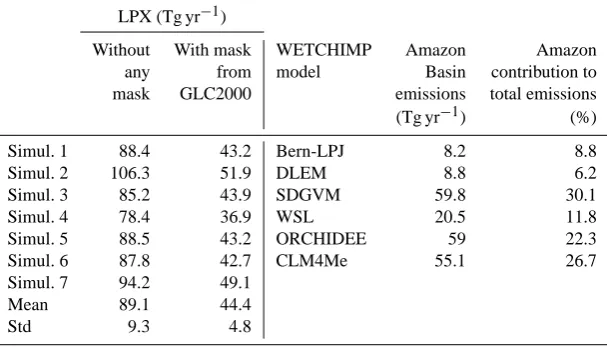
uncertain-ties. In particular, uncertainties in floodplain extent (i.e., difference between GLC2000 and PCR-GLOBWB output) modulate the simulated emissions by a factor of about 2. Our best estimates, using PCR-GLOBWB in combination with GLC2000, lead to simulated Amazon-integrated emissions of 44.4±4.8 Tg yr−1. Additionally, the LPX emissions are highly sensitive to vegetation distribution. Two simulations with the same mean PFT cover, but different spatial distri-butions of grasslands within the basin, modulated emissions by about 20 %. Correcting the LPX-simulated NPP using MODIS reduces the Amazon emissions by 11.3 %. Finally, due to an intrinsic limitation of LPX to account for season-ality in floodplain extent, the model failed to reproduce the full dynamics in CH4emissions but we proposed solutions to
for, but still remains lower than in most of the WETCHIMP models. While our model includes more mechanisms spe-cific to tropical floodplains, we were unable to reduce the uncertainty in the magnitude of wetland CH4emissions of
the Amazon Basin. Our results helped identify and priori-tize directions towards more accurate estimates of tropical CH4emissions, and they stress the need for more research to
constrain floodplain CH4emissions and their temporal
vari-ability, even before including other fundamental mechanisms such as floating macrophytes or lateral water fluxes.
1 Introduction
Methane (CH4) is an important atmospheric component
be-cause of its contribution to radiative forcing and its role in atmospheric chemistry. Its chemical interactions result in indirect radiative forcings through its impacts on the oxi-dizing capacity of the atmosphere, and the production of tropospheric ozone and stratospheric water vapor. Wetlands contribute between one-quarter and one-half of global CH4
emissions (Kirschke et al., 2013). However, both the global magnitude and the latitudinal distribution of wetland emis-sions are poorly known (e.g., Denman et al., 2007). Tropi-cal (30◦N–30◦S) wetlands are estimated to represent about 50 % of the natural wetland CH4 emissions. In addition,
tropical wetlands also contribute to the variability in atmo-spheric CH4 concentration at different timescales, ranging
from glacial–interglacial cycles (Loulergue et al., 2008; Sin-garayer et al., 2011, Baumgartner et al., 2012) to the cur-rently observed year-to-year variability (e.g., Bousquet et al., 2006).
To estimate regional to global emissions of CH4, two
mod-eling strategies are commonly applied: the top-down and the bottom-up approach. The top-down approach, also re-ferred to as atmospheric inverse modeling, optimally com-bines atmospheric observations of CH4, a model of
atmo-spheric chemistry and transport, and a priori information about sources and sinks (e.g., Bergamaschi et al., 2009; Bousquet et al., 2006, Monteil et al., 2011). The bottom-up approach integrates the available information about wetland CH4emissions at the process level into regional (Bohn et al.,
2007) and global terrestrial models (e.g., Riley et al., 2011; Ringeval et al., 2011). The two approaches are complemen-tary, in that they address different spatial scales and are con-strained by observations relevant to different parts of the CH4
budget. Top-down estimates provide only limited insight into the underlying biogeochemical processes controlling emis-sions, particularly over regions where several processes and sources overlap. In contrast, the bottom-up approach incor-porates knowledge of small-scale processes, but extrapola-tion of their local emission estimates to larger scales com-patible with the atmospheric signals is uncertain. Top-down and bottom-up approaches are usually not independent since
the top-down approach often uses bottom-up emission maps as an a priori estimate (e.g., Spahni et al., 2011). Due to the current limitations of each approach (see e.g., Houweling et al., 2013 about top-down models), the uncertainties after combining them are still large. This applies to both the size of global wetland emissions and their year-to-year variabil-ity (Kirschke et al., 2013). Despite these uncertainties, the Amazon watershed has been identified as a key player in the mismatch between top-down and bottom-up estimates (Pi-son et al., 2013). For instance, the magnitude of the Amazon wetland CH4emissions increases from 44 to 52 Tg CH4yr−1
when CH4retrievals from a remote-sensing instrument (e.g.,
SCIAMACHY) are implemented as constraints in the inverse modeling system of Bergamaschi et al. (2009).
Both SCIAMACHY CH4 concentrations and airborne
measurements (Beck et al., 2012; Miller et al., 2007) showed elevated concentrations over the Amazon, but attributing these high concentrations to specific sources (e.g., wetlands) is not straightforward. In recent years, potentially important - but still-debated new mechanisms of CH4 production
un-der oxic conditions (see e.g., Keppler et al., 2006; Nisbet et al., 2009; Vigano et al., 2008) or anoxic conditions (Covey et al., 2012) have been proposed. Nonetheless, recent isotope analysis showed that the majority of airborne measured CH4
concentration elevations can be attributed to microbial CH4
production (Beck et al., 2012), reducing the number of poten-tial drivers of the observed elevated concentrations. Despite possible alternative sources of CH4 in the Amazon Basin,
wetlands thus likely remain the main source of the Amazon CH4emissions.
Melack et al. (2004) estimated the Amazon-Basin-integrated wetland emissions at 22 Tg yr−1 by combining
flux measurements and remotely sensed wetland distribu-tions. However, a large fraction of the spatio-temporal vari-ability in the processes that control the CH4emissions are not
accounted for in this approach, which introduces large uncer-tainties. The use of land surface models (LSMs) (e.g., Riley et al., 2011) is a promising approach for reducing the un-certainties further. However, the recent WETCHIMP LSM intercomparison experiment (Melton et al., 2013; Wania et al., 2013) shows a large range of estimates for the tropics, indicating that tropical wetlands are poorly represented in these models. This is partly explained by the absence of a dedicated parameterization of tropical wetland ecosystems in the current generation of LSMs, affecting both the estimated wetland extent and CH4flux densities (i.e., the flux per m2of
wetland). Parameterizations introduced in LSMs to simulate the wetland CH4flux densities are primarily representative
floodplains, which is the main habitat associated with wet-land in the Amazon watershed (Hess et al., 2003; Miguez-Macho and Fan, 2012). Further development of LSMs is ur-gently needed to account for these omissions, given the im-portance of tropical wetlands for understanding global CH4.
In the present study, we present the first adaptations of a global process-based model of CH4 emissions to Amazon
floodplains specificities. This provides in the first step to-wards a more realistic model for tropical wetlands. We do this in the framework of the LPX-Bern 1.0 Dynamic Global Vegetation Model (Land surface Processes and eXchanges, Bern version 1.0) (Spahni et al., 2013; Stocker et al., 2013) given its ability to simulate transitions of vegetation types, carbon and water pools between different terrestrial ecosys-tems. LPX includes a parameterization for the simulation of boreal peatland emissions developed by Wania et al. (2010). Besides, wetland CH4emissions were estimated in LPX for
remotely sensed wetland extents (Prigent et al., 2007) by us-ing simple parameterizations (Spahni et al., 2011, Wania et al., 2013). We adapted the Wania et al. (2010) process-based approach to the case of the Amazon floodplains. To do so, we used the outputs of a hydrological model (PCR-GLOBWB) to prescribe the floodplain extent in the LPX model. The LPX model was extended with a representation of the Amazon floodplain vegetation, focusing on the contributions of trees and grasses to vegetation cover and productivity. The model extended with floodplains and floodplain CH4 is tagged as
LPX-Bern version 1.1. The different parameterizations were tested using remote-sensing data (GLC2000, MODIS), in situ flux measurements and results of the WETCHIMP model intercomparison (Melton et al., 2013; Wania et al., 2013). The model was used to estimate the sensitivity of the CH4
emissions from the Amazonian floodplains to different (un-certain) processes. The comparisons with observations and sensitivity tests allowed identifying and prioritizing the chal-lenges faced to obtain more accurate estimates of Amazon CH4emissions.
Section 2 describes the use of PCR-GLOBWB-simulated floodplains extent, the representation of floodplain vegeta-tion and associated CH4emissions and the sensitivity
analy-ses. The main results are presented in Sect. 3. Model perfor-mance, uncertainties and priorities for future developments are discussed in Sect. 4.
2 Methods
2.1 The base LPX model
The LPX-Bern 1.0 (hereafter LPX) is a subsequent develop-ment of the Lund-Potsdam-Jena (LPJ) dynamic global vege-tation model (Sitch et al., 2003), which combines process-based, large-scale representations of land–atmosphere car-bon and water exchanges and terrestrial vegetation dynamics in a modular framework. In the following, we briefly present
the LPX characteristics relevant to understand the modifica-tions described in Sects. 2.2 to 2.5 to improve estimates of CH4emissions from the Amazonian basin.
2.1.1 Vegetation representation
In LPX, following Wania et al. (2009b), boreal (>45◦N) grid cells are treated either as peatland or as mineral soil de-pending on the soil carbon content derived from Tarnocai et al. (2009). The computation of water and carbon fluxes dif-fers between these soil types. In particular, peatland soils are vertically separated into the acrotelm and the permanently water-saturated catotelm. This separation is not relevant for floodplains and therefore, floodplains are treated as mineral soils (see Sect. 2.2.1). Plant hydrology is treated following Gerten et al. (2004) with an extension of the number of min-eral soil layers to eight following Wania et al. (2009b).
Each mineral grid cell of LPX is split into fractions (here-after land units, LUs). LUs are reserved for natural vegeta-tion, agriculture (including cropland and pasture), and built-up areas (Strassmann et al., 2008). Peatlands are modeled as a separate LU (Spahni et al., 2013). The natural vegetation LU consists of 10 generic plant functional types (PFTs) that may co-exist. Peatland LUs may contain any of these generic PFTs, complemented by two peatland-specific PFTs intro-duced by Wania et al. (2009a): flood-tolerant C3 graminoids (sedges) and Sphagnum mosses. Within a given LU, it is as-sumed that the different PFTs are well mixed. As a result, the PFTs compete locally for resources while different LUs in the same grid cell are assumed to occupy different environ-ments, without competition of PFTs among them. To model Amazon floodplains, we introduced a new LU as well as new flood-tolerant PFTs (see Sects. 2.2 and 2.3).
The fundamental entity simulated in LPX is the average in-dividual of a PFT. Each PFT is characterized by its own set of parameters describing growth, carbon uptake, etc. Photosyn-thesis and water balance are coupled in a two-step approach. First, LPX calculates the non-water-stressed photosynthesis rate, and then optimizes the canopy conductance based on water-limited transpiration (Sitch et al., 2003). Contrary to most of the commonly used global vegetation models (e.g., see Krinner et al., (2005) for the ORCHIDEE model), there are no PFT-specific parameters for the optimal maximum rubisco-limited potential photosynthetic capacity (vcmax) and
the potential rate of Ribulose-1,5-bisphosphate (RuBP) re-generation (vjmax). This has an effect on our strategy to model
flood tolerance for the newly introduced PFTs.
at the end of each simulation year. Such reductions can be caused by depressed growth efficiency, heat stress, nega-tive NPP and by exceeded PFT-specific bioclimatic limits. For a realistic simulation of floodplain vegetation cover, tree mortality required specific attention, as will be described in Sect. 2.3.3.
In addition, two rules control the coexistence of grasses vs. trees in a LU of a given grid cell (Sitch et al., 2003), which plays a key role in our study: (i) self-thinning of woody veg-etation (i.e., a reduction in the population) if the LU FPC sum of woody vegetation exceeds an arbitrary limit of 95 %, (ii) competitive dominance of taller-growing woody PFTs by first reducing herbaceous PFT biomass if tissue growth leads to a grid-cell FPC sum greater than unity.
Finally, note that for this study dynamical nitrogen cycling (Stocker et al., 2013; Spahni et al., 2013) has been turned off. 2.1.2 Wetland CH4emissions
Wetland CH4 emissions are the product of the wetland
ex-tent and the CH4flux density. In LPX, natural wetland CH4
emissions are computed for different classes of wetlands: bo-real peatland, inundated wetland and wet mineral soils. Orig-inally, for peatland CH4emissions, an additional scaling
fac-tor was used to account for the peatland microtopography (see Wania et al., 2010; Zürcher et al., 2013). In the present study, such a scaling procedure is not used for tropical flood-plains (see Sect. 2.5).
The areal extents of boreal peatlands and inundated wet-lands are derived from different maps: soil survey maps de-rived from Tarnocai et al. (2009), Yu et al. (2010) and Wania et al. (2012) for peatlands and maps of remotely sensed in-undation extent given by Prigent et al. (2007) for inundated wetland. The extent of wet mineral soils is defined as the grid-cell fraction that is not occupied by peatland and inun-dated wetland (and rice), but for which the soil water content is above a given threshold (Spahni et al., 2011). Originally, in LPX, floodplains were included in the inundated wetland class and thus, the extent was not explicitly defined but de-rived from Prigent et al. (2007). In our approach, however, the floodplain extent is prescribed using outputs of the PCR-GLOBWB model (see Sect. 2.2.1).
In previous studies (Spahni et al., 2011; Wania et al., 2010), process-based computation of CH4flux densities were
restricted to the case of boreal peatlands. CH4flux densities
for inundated wetland and wet mineral soils were estimated using scaling factors, such as the simple CH4/ CO2ratio and
CO2heterotrophic respiration (HR) (Spahni et al., 2011;
Wa-nia et al., 2013). A similar approach is used in the LPJ version of Hodson et al. (2011).
In the case of boreal peatlands, the CH4flux density that
escapes to the atmosphere results from three processes: pro-duction, oxidation and transport. Water saturation and O2
concentration are key variables for estimating the balance be-tween production and oxidation and thus the resulting CH4
concentration in each soil layer. The O2 transport by
diffu-sion and through plants is explicitly represented in the model. In Wania et al. (2010), the potential carbon pool for methano-genesis is estimated from the heterotrophic respiration (HR). Part of the NPP is attributed to root exudates, which con-tributes to HR without passing through the litter and soil pools. The potential carbon pool for methanogenesis is dis-tributed over all soil layers, weighted by the root distribu-tion. This carbon is split into CH4 and CO2 depending on
a (fixed) maximum ratio and the anoxic status of each soil layer. The anoxic status of each soil layer is computed in LPX as a function of the local soil water content rather than the actual O2concentration. The dissolved CH4
concentra-tion and the gaseous CH4 fraction are calculated from the
amount of CH4available in each layer. The rate of CH4
ox-idation is computed as a function of the O2 concentration.
Remaining dissolved CH4escape to the atmosphere by
dif-fusion either through the soil (saturated or not) or through plant tissue pores (aerenchyma). Gaseous CH4escape to the
atmosphere by ebullition. Thus, as in Wania et al. (2010), a total of three transport processes is accounted for: diffu-sion, plant-mediated transport and ebullition. The ebullition parameterization makes use of the partial pressure of CO2for
triggering ebullition events, following (Zürcher et al., 2013). Our modifications mainly consist of accounting for the O2
concentration to compute the anoxic status of soil layers and removal of the catotelm/acrotelm distinction in the tropical zone (see Sect. 2.5).
2.2 Floodplain hydrology
2.2.1 Floodplain extent
Global wetlands vary widely in hydrologic, soil and vege-tation characteristics. Floodplains differ fundamentally from other wetland types, such as bogs, mires and fen, which depend on local precipitation and groundwater fluctuations (Mistch and Gosselink, 2000). Floodplains result from tem-porarily increased river discharge, importing sediment and nutrients from elsewhere. Instead, floodplains tend to have mineral soils and can sustain productive vegetation. The Amazon Basin covers 7 million km2, with floodplains as the dominant type (Hess et al., 2003; Miguez-Macho and Fan, 2012).
In the Amazon Basin, this new floodplain LU grows or shrinks over time mainly in exchange with the natural vege-tation LU, hereafter referred to as the non-floodplain LU. The hydrological conditions (annual-mean extent and seasonally varying water depth) in the LPX floodplain LU are prescribed according to the outputs of PCR-GLOBWB. This hydrolog-ical model includes a river-routing routine capable of simu-lating the hydrology of floodplains (Van Beek and Bierkens, 2009; van Beek et al., 2011). A similar approach using PCR-GLOBWB has been used in the PEATLAND-VU model for simulation of CH4 emissions from northern wetlands
(Pe-trescu et al., 2010). The use of a hydrological model instead of remote-sensing measurements (e.g., Papa et al., 2010) al-lows us to represent the two components of the wetland CH4
emissions (flux density and wetland extent), which can be ap-plied to years for which no inundation data are available. The simulation of floodplain extent may introduce potential bi-ases, in particular because evaluation of model performances is difficult for the Amazon Basin (cf. Discussion).
PCR-GLOBWB is a global hydrological model and has been developed primarily for estimating the availability of fresh water (also called “blue” water) (van Beek and Bierkens, 2009; van Beek et al., 2011; Gleeson et al., 2012). PCR-GLOBWB calculates the water storage on a cell-by-cell basis in two vertically stacked soil layers and an un-derlying groundwater reservoir on a daily time step. The exchange between the soil column and the atmosphere in-cludes rainfall, snowmelt and evaporation from plants and interception. The soil column produces runoff, comprising direct surface runoff, subsurface storm flow and base flow, which is routed as discharge along the drainage network us-ing the kinematic wave approximation for channels. Where interrupted by lakes or reservoirs, parameterized on the basis of the GLWD1 (Lehner and Döll, 2004), discharge is con-trolled by storage–outflow relationships, including a prog-nostic operation scheme that optimizes the release of each reservoir (van Beek et al., 2011). In each grid cell containing a river channel, floodplains can form if the simulated channel storage exceeds the capacity at bank-full discharge. The re-sulting floodplain area and inundation depth follow from the distribution of elevations above the river bed, which is pa-rameterized using the cumulative land area in a cell (subdivi-sions of 0.01, 0.05 and 0.1 through 1.0 by increments of 0.1). The basis of this subdivision is the HYDRO1k (http://gcmd. nasa.gov/records/GCMD_HYDRO1k.html) which provides a global, hydrologically correct elevation data set with a spa-tial resolution of 1×1 km2. The height of the floodwaters (hereafter “flooding depth”) and the extent of the sub-merged area thus follow from intersecting the cumulative floodplain volume with the discharge in excess of channel storage. In terms of variables, for a given daytand a given grid cell, the total volume that is stored in a channel reach of a grid cell (wst), the resulting floodplain extent (fldf) and the flooding depth aboveground (fldd) are given by PCR-GLOBWB. The fldd given by PCR-GLOBWB is always positive or null. The
river channel area is subtracted a posteriori from fldf, while the river channel volume is subtracted from wst. Contrary to the earlier application of PCR-GLOBWB to estimate CH4
emissions over northern wetlands (Petrescu et al., 2010), the extent of the floodplain is computed here online, leading to a dynamic interaction between floodplain extent and depth and flood wave propagation as a result of increased resistance compared to bank-full discharge (Winsemius et al., 2013).
In LPX, the annual extent of the floodplain LU per grid cell (fldfmean) is defined as the area that corresponds to the annual mean flood volume (wst) as calculated by PCR-GLOBWB (cf. Fig. A1, top and middle panels for an ex-ample). Because only two LUs are considered in the present study, changes in the floodplain LU extent are balanced by corresponding changes in the non-floodplain LU.
2.2.2 Flooding depth seasonality
The Amazon Basin is characterized by a period of more fre-quent rain (approximatively from February through April) and a period of less intense rainfall, with the driest period between July and September. This leads to large water level fluctuations and thus seasonality in both floodplain extent and flooding depth. The river level lags behind the seasonal pattern of precipitation by a few months because of storage of water in different water pools (see e.g., Fig. 1 of Bartlett et al., 1990). The Amazon River is mainly monomodal, that is, characterized by a single pulse of flooding per year, contrary to other basins in South America.
As for peatland (Wania et al., 2009b), we computed a water table position (WTP) variable for the floodplain LU. For a given time step, depending on the value of the PCR-GLOBWB-derived flooding depth that is prescribed to LPX (flddLPX), two cases arise:
– if flddLPX is equal to 0, the LPX-computed soil
wa-ter content is used for the WTP calculation. In this case, WTP is negative, and equal to the difference (ex-pressed in meters) between the maximum and actual soil water content.
– if flddLPXis positive, the soil water content is set to full
saturation over the floodplain LU and flddLPXis used
as WTP.
The PCR-GLOBWB-derived flooding depth is consistent with a seasonally varying floodplain extent. In contrast, the simulation of vegetation growth and distribution in LPX is calculated for an annually constant floodplain fraction (fldfmean). Therefore a method is needed to calculate flddLPX,
a) GLC2000 flooded
vegetation b) PCR-GLOBW floodplains
(-) 0.90
0.70
0.50
0.30
0.10 0.06 0.02 –
–
–
–
[image:6.595.116.484.73.343.2]– – –
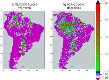
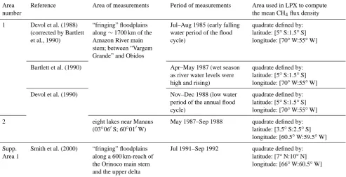
Fig. 1. Fraction of total grid cell at 0.5◦resolution (unitless) covered by (a) flooded vegetation as defined by GLC2000 and (b) floodplain given by PCR-GLOBWB (mean annual value over 1979–2009 of fldfmean). The (b) panel map is used as input of LPX for simulations
without year-to-year variability of floodplain extent (simulations 1–6 in Table 5).
proportional to the product of flood depth and flood fraction. This differs from the flood volume, because floodplains have a nonuniform depth. On the other hand, the floodplain LU in LPX has a uniform depth. Approach 2 is a sensitivity test to evaluate the importance of this inconsistency.
In the redist approach, for a given day t and grid cell, flddLPX= flddredistwhere flddredistwas defined as follows:
If wst(t )≥wst,flddredist(t )=fldd+
wst(t )−wst fldfmean
If wst(t ) <wst, flddredist(t )=fldd·
wst(t )
wst ,
(1)
with wst, fldd, fldf respectively in m3, m and m2. Over-lined variables denote annual means.
In the product case, flddLPX=flddproductas computed in a
given year by
If fldf(t )≤ fldfmean,flddproduct(t )= fldd(t )· fldf(t )
If fldf(t ) > fldfmean, flddproduct(t )= fldd(t ).
(2)
The two cases (Eqs. 1 and 2) are displayed for a given grid cell in Fig. A1 (bottom panel). The seasonal cycle of flddredist
and flddproduct over the whole Amazon Basin are given in
Fig. A2. In both cases, a large proportion of the horizontal seasonality (i.e., the seasonality in wetland extent) is
trans-ferred into the seasonality of the flooding depth. The season-ality in wetland extents is assumed to be a major driver of the variability in wetland CH4 emissions (Bloom et al., 2010;
Ringeval et al., 2010). There are no observations on flood-ing depth available at large scale. However, we compared the simulated flooding depth to information available on partic-ular sites (Sect. 2.6.3 and Fig. A4). In addition, the effects of the seasonality in the floodplain extent on the simulated CH4
emissions is evaluated in Sect. 3.3 and discussed in Sect. 4. 2.3 Floodplain vegetation
As mentioned in Sect. 2.1.2, heterotrophic respiration is used as a proxy for the potential carbon pool for methanogene-sis, including contributions from litter/soil carbon and root exudates. In equilibrium, and without accounting for fire-related fluxes, heterotrophic respiration is in balance with NPP. To get NPP right requires a realistic representation of the floodplain vegetation carbon balance in the Ama-zon Basin. Note also that the vegetation type and structure are important since they influence the CH4 transport
path-way from the soil to the atmosphere (diffusion/ebullition vs. plant-mediated transport).
flood-related stress on productivity in the model. In addi-tion, we changed the mortality parameterization for trees in the floodplain LU. The aim of these modifications was to improve the representation of (i) the fractional cover-age of grasses versus trees and (ii) the floodplain NPP. The grasses/trees contribution to total vegetation was evaluated against the GLC2000 data set. Floodplain NPP was evaluated against MODIS-derived NPP in combination with GLC2000 (see Sect. 2.6.1).
2.3.1 Flood-tolerant tropical PFTs
The original model version accounts for three tropical PFTs: tropical leaved evergreen (TrBE), tropical broad-leaved raingreen (TrBR) and C4 grasses (C4G). This ap-proach was extended by defining three new PFTs, which are flood-tolerant versions of the existing tropical PFTs, increas-ing the total number of natural PFTs in LPX from 10 to 13. 2.3.2 Photosynthesis
The flooding of vegetation causes anoxic conditions in the rooting zone, which causes accumulation of ethylene within plants, and lower redox potentials. Eventually, phytotoxins accumulate in the rooting zone, impeding plant growth. To account for this inundation stress, we modified the anoxic stress factor on productivity as introduced by Wania et al. (2009a). The introduced parameterizations are empirical relations to mimic the influence of inundation stress on veg-etation productivity and distribution in order to bring these properties into a realistic range. Chosen formulations are similar to Wania et al. (2009a). In a next step, the LPX model could be more deeply modified to be more mechanis-tic (see Sect. 4). Here, as in Wania et al. (2009a), two PFT-specific parameters are used, namely, a threshold water table (WTPmax), above which a PFT experiences inundation, and
a maximum survival duration of inundation (tinund), which
counts how many days a PFT can survive under inundation. Thus, for a given dayd and a given PFT,
If WTP(d)≥ WTPmax,icount(d)
=min(tinund,icount(d−1)+1)
If WTP(d) < WTPmax,icount(d)=0.
(3)
The monthly gross primary production is reduced by icount/tinund where icount is the monthly mean value of
icount(d). We assumed that one day with WTP below WTPmaxis sufficient to reset the stress to 0. Contrary to
Wa-nia et al. (2009a), the icount variable is not reset to 0 at the beginning of each month in order to avoid unwarranted in-fluences of the division of a year into months, and has an upper limit (tinund) to limit the range of icount/tinundbetween
0 and 1. As in Wania et al. (2009a), the monthly respiration is reduced by this scaling factor.
Besides, the growth of flood-tolerant PFTs is reduced un-der drought-stress, following treatment of flood-tolerant C3
graminoids in Wania et al. (2009b). As soon as WTP drops below −20 cm, flood-tolerant PFTs experience stress and GPP is reduced proportional to WTP by a factor ranging from 0 to 1 for WTPs between [−20 cm,−40 cm]. Below−40 cm, the stress is equal to 1, corresponding to a primary produc-tion of 0.
The GPP of flood-tolerant PFTs in the non-floodplain LU is reduced as well. A simplified approach is taken, inde-pendent of the hydrological conditions encountered in the non-floodplain LU. The prescribed stress corresponds to the drought stress in the floodplain LU at a WTP of−25 cm. This way, the flood-tolerant PFTs are effectively outcompeted by classical PFTs and the impact of flood-tolerant PFTs on the non-floodplain classical “natural” LU is limited.
To parameterize the flood-tolerant PFTs, we chose rep-resentative values for graminoids and flood-tolerant forest trees. While such representative values will never be able to represent the high variability in flooding susceptibility of this diverse ecosystem (Junk and Piedade, 1993; Piedade et al., 2010), we chose a value for emergent C4 grasses with high productivity, dominating the herbaceous Amazon ecosystem, like Echinochloa polystachya and Paspalum repens. In our approach, we did not account for floating macrophytes (e.g., Paspalum fasciculatum) whose specificities (Wassmann et al. 1992) would require a more fundamental recoding of LPX (see Discussion). Nevertheless, the sensitivity of CH4
emissions to key characteristics of floating macrophytes (no plant-mediated transport and no exudates) will be tested in Sect. 2.6.3. Amazon floodplain water is turbid, and in tur-bid water the submerged grasses cannot photosynthesize. Plant species, such as Echinochloa polystachya, are char-acterized by high productivity and long shoots to maintain leaves above the water. The higher production potential of C4 as compared to C3 plants may explain the dominance of C4 plants in tropical floodplains (Piedade et al., 1991). Piedade et al. (1991) report shoots longer than 10 m (see Fig. 1 of Piedade et al., 1991).
The most commonly encountered species of trees are Lae-tia corymbulosa (evergreen), Crataeva benthamii (decidu-ous) and Pseudobombax munguba. Most trees species oc-cur both in flooded and in non-flooded ecosystems, ex-cept for some species, such as Pseudobombax munguba, which is stem-succulent. Trees are characterized by re-duced metabolism during the aquatic phase (Wittmann et al., 2006). Forests tolerate extended periods of flooding, up to 270 d yr−1(Wittmann et al., 2002).
Following these descriptions, we chose a higher WTPmax
for flood-tolerant grasses than for flood-tolerant trees, and the opposite pattern fortinund (i.e., longer for flood-tolerant
for the impact of submergence. Unfortunately, there are no direct observations available to describe how flood duration and flooding depth affect productivity for PFTs in tropical floodplains. Instead, we evaluated the sensitivity of vegeta-tion dynamics and productivity to these parameter settings (see Sect. 3.2). Note also that given values of (WTPmax,
tinund) will have a different effect on vegetation dynamics
and productivity depending on the chosen flooding depth de-scription (i.e., flddproductor flddredist). Negative WTPmax
val-ues (between−100 and −300 cm as in Wania, 2007) were assigned to non-tolerant PFTs, ensuring that flood-tolerant PFTs are more adapted to flooded conditions. 2.3.3 Tree mortality
Mortality corresponds to a reduction in population density and is computed at a yearly timescale (Sitch et al., 2003). Mortality can occur as a result of light competition, a nega-tive annual carbon balance, heat stress or when bioclimatic limits of a PFT are exceeded for an extended period (Sitch et al., 2003). A new mortality term was introduced to repre-sent reduction in population density of flood-tolerant trees in the floodplain LU. This mortality term represents enhanced tree mortality, even of adapted trees upon flooding (Bailey-Serres and Voesenek, 2008). A constant additional mortality for flood-tolerant trees at flooding, hereafter calledMadd, is
chosen and is used as a tuning parameter (see the next sec-tion).
2.3.4 Soil carbon decomposition
As for peatlands (Wania et al., 2009a), the sensitivity of car-bon decomposition to soil water content (Rmoist) was set to
a constant value. While the WTP could occasionally fall be-low the soil surface (see Sect. 2.2.3), the floodplain LU soil remains almost always saturated, justifying this approach. Under anoxic conditions, decomposition is slow because anoxia limits phenol oxidase activity and causes phenolic compounds to accumulate. For peatlands,Rmoistof 0.35 was
used. For floodplains, an arbitraryRmoistof 0.5 was chosen
to account for a faster anaerobic degradation in floodplains than in peatlands due to a more neutral pH. The CH4
emis-sions sensitivity toRmoistis discussed in Sect. 4. 2.4 Year-to-year variability in floodplain extent
In regional simulation 7 (see Sect. 2.6.3), interannual varia-tion in floodplain extent was accounted for as forced by PCR-GLOBWB outputs. This leads to the conversion of land from one LU (called hereafter lu2) to the other LU (lu1) and of the
various PFTs accordingly. All variables describing soil and vegetation were converted from one LU to the other. Non-floodplain and Non-floodplain LU classes use the same PFTs; however, they behave differently in each LU. For any tree PFT of the expanding LU lu1, the properties (biomass, LAI,
crown area, hereafter called variablesV) of a tree individual
were modified according to Eq. 4. This equation describes the transfer of any variableV of a given PFTa in lu1from
yeart to yeart+1:
V (PFTlu1,a, t+1)=
V (PFTlu1,a,t )·A(lu1,t )·n(PFTlu1,a,t )+P
b∈L
1A·V (PFTlu2,b,t )·n(PFTlu2,b,t )
A(lu1,t+1)·n(PFTlu1,a,t+1) ,
(4)
with1A=A(lu1, t+1)−A(lu1, t ) >0, and where, at time
t,A(luX, t) is the extent of the luX LU;n(PFTY, t) is the
number of individual trees for the PFTY, andL is the list
of PFTs in lu2 “corresponding” to PFTlu1,a. Indeed, each
PFT is characterized by a rank defining it among the 13 pos-sible PFTs (second subscript corresponding to, e.g., TrBE, TrBR, C4G, flood-tolerant TrBR, etc.) and the LU in which it grows (first subscript corresponding to floodplains or non-floodplains). As a first approach, we chose to make each PFT correspond to the same PFT of the other LU (i.e.,L= {a}in Eq. 4). For instance, if the floodplain LU shrinks (lu2= luflood
in Eq. 4), TrBR of the floodplain LU is converted into TrBr of non-floodplain LU. The modifications introduced in LPX to simulate floodplains alter the forest characteristics: for exam-ple, floodplain forests are characterized by a large number of small trees, while non-floodplain forests consist of a smaller number of larger trees. Due to these differences, any conver-sion from one LU to the other leads to a high mortality in the tree population. This can happen for flood-tolerant PFTs that experience stress on the classical natural LU when floodplain extent shrinks.
The different litter and soil carbon pools, as well as the number of individual trees after conversion of a given frac-tion of lu1to lu2, were computed following an equation
simi-lar to Eq. 4. However, these variables were not computed for the average individual in the model and thus no weighting by the number of individuals is necessary. Instead, a simple mean of the given variables of two corresponding PFTs was taken and weighted by the extent of lu1and1A. Finally, in
the first attempt, the LU conversion did not account for redis-tribution of water in order to prevent any major modifications in the non-floodplain LU.
2.5 Extension of the LPX CH4module to floodplains
Since the main processes leading to CH4 emissions
(pro-duction, oxidation and transport) are common to all wet-lands, only a limited number of modifications of the origi-nal CH4 emission routine were needed in order to adapt it
for floodplain CH4emissions. Except for the introduction of
a methanogenesis reduction in the presence of O2, which is
considered a generic process-based improvement, all other modifications were needed to make the CH4routine
consis-tent with the implemented LPX representation of floodplain vegetation.
In Wania et al. (2010), the potential carbon pool for methanogenesis is split into CO2 and CH4 as function of
(hereafter calledrCH4/CO2and equal to 0.10), and (ii) the
de-gree of anoxia of each soil layer. The dede-gree of anoxia of each soil layer is computed by using the soil water content: 1−fair, wherefairis the fraction of air in each layer. Here we
introduce a decrease of methanogenesis in the presence of O2
in such a way that the degree of anoxia is now approximated by
anoxia =1−
fair+(1−fair)·
[O2]
[O2]eq
, (5)
where [O2] is the computed and dissolved O2concentration
of the given soil layer and [O2]eqis the dissolved
concentra-tion that is in Henry’s equilibrium with the atmosphere. This modification makes the anoxia computation related to the oxygen concentration (and not to air fraction alone), which is more in agreement with basic knowledge about methano-genesis (Conrad et al., 1989).
As underlined in previous sections, we treated floodplains as mineral soils in LPX. That means that no distinction be-tween catotelm/acrotelm was made in the floodplain LU. Also porosity was based on a soil texture map as for other mineral soils instead of using constant porosity and mini-mum gas fraction for peatlands as in Wania et al. (2010). No thresholds on porosity were applied to allow ebullition. All flood-tolerant PFTs contribute to methanogenesis sub-strate. However, only the flood-tolerant C4 plants contribute to plant-mediated transport. Root distribution with depth is kept as in Wania et al. (2010). Note also that, as in Wania et al. (2010), the water column above the soil surface is added to the top soil layer, even though this is less appropriate for large flooding depths (see discussion).
Table A1 summarizes the meaning of main vari-ables/parameters introduced in LPX.
2.6 Experimental set-up and data sets used for evaluation
2.6.1 Floodplain extent
As outlined above, we defined the annual extent of the flood-plain LU per grid cell (fldfmean) as the area that corresponds to the annual mean flood volume (wst) as calculated by PCR-GLOBWB (cf. Fig A1, top and middle panels for an exam-ple). PCR-GLOBWB was implemented on a spatial grid of 0.5◦at a daily time step. For these simulations, we made use of the ERA-Interim reanalysis (Dee et al., 2011) to force the model with precipitation, temperature and reference poten-tial evapotranspiration over the period 1979–2009, for which the fields were gridded at the required spatial and tempo-ral resolution. This reanalysis data set has limited qualities in reproducing the hydrological cycle, mainly because pre-cipitation is not included in the data assimilation scheme. Therefore, a scaled precipitation product was chosen which corrects the ERA-interim precipitations using the GPCP ob-servational data set (Balsamo et al., 2011). This correction,
however, is coarse (2.5 degrees), resulting in a relatively poor performance over highly variable terrain. Therefore, as an ad-ditional correction, all forcing variables (precipitation, evap-otranspiration and temperature) were scaled to bring their long-term means in accordance with the CRU TS 2.1 (New et al., 2002). This correction was applied on a month-by-month basis for time period of the CRU data set (1971–2001) and regions where stations were available.
The model was spun-up by iteratively updating the long-term components of the groundwater system over a period of 10 years followed by a transient simulation. This was then repeated by a full run over the entire simulation period to initialize the stores of the routing model (channels, reservoirs and lakes). This simulation strategy closely follows that of Van Beek et al. (2011), who used the CRU TS2.1 data set directly to force the model. Although different climatological data were used, the long-term means over gauged areas are similar. Therefore, the validation exercise undertaken by Van Beek et al. (2011) and the limitations that were found are expected to apply to our model as well.
To evaluate the land cover as simulated using the combined LPX–PCR-GLOBWB set-up, we made use of the Global Land Cover 2000 (GLC2000 hereafter) land cover map (http://bioval.jrc.ec.europa.eu/products/glc2000/ products.php). GLC2000 is based on multi-resolution satel-lite data (combining 4 independent data sets) and pro-vides the dominant vegetation type, among 40 classes, for each 0◦0032.144400latitude×0◦0032.144400longitude grid cell. We made use of the regional data set for South America (The Land Cover Map for South America in the Year 2000, 2003).
To compare to PCR-GLOBWB, for each 0.5×0.5◦grid
cellg, the floodplain extent was estimated by counting all GLC2000 grid cells at GLC2000 resolution within g cov-ered by any of the following vegetation classes: “fresh water flooded forests”, “permanent swamp forests”, “periodically flooded shrublands” or “periodically flooded savannah”. The GLC2000 class “water bodies” was not used, since it rep-resents lakes and water channels, rather than floodplains. Floodplain fractions were compared to the long-term mean (i.e., 1979–2009) fldfmean.
2.6.2 Floodplain vegetation
Three LPX simulations were performed at 0.5◦ resolution with different sets of values for fldd, WTPmax, tinund and
Madd (Table 1). For each simulation, the Climate Research
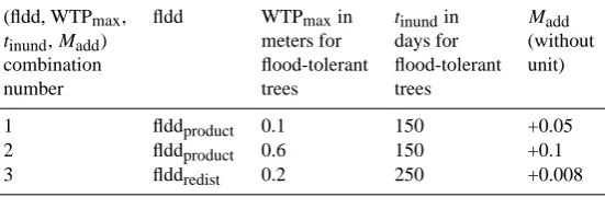
Table 1. Different combinations of (fldd, WTPmax,tinundandMadd). Only the values of (WTPmax,tinund,Madd) for flood-tolerant trees
vary from one simulation to the other. For all simulations, (WTPmax,tinund) for flood-tolerant grasses are set to (10 m, 10 days).Maddhas a
meaning only for tree PFTs (no population density for grass PFTs).
(fldd, WTPmax, fldd WTPmaxin tinundin Madd
tinund,Madd) meters for days for (without
combination flood-tolerant flood-tolerant unit)
number trees trees
1 flddproduct 0.1 150 +0.05
2 flddproduct 0.6 150 +0.1
3 flddredist 0.2 250 +0.008
data for the 1901–1931 period. Then, a transient run was performed for the 1931–2009 period. In the Results section, we focus on the 1990–2009 period. For all simulations, ex-cept for regional simulation 7 (see Sect. 2.6.3), both spin-up and transient runs were performed without IAV in the flood-plain LU extent. Thus, the 1979–2009 climatology of PCR-GLOBWB outputs was used to prescribe floodplain extents. Note that the climate data sets used to force LPX and PCR-GLOBWB are not the same. The correction of ERA-Interim to CRU TS 2.1, described in the previous section, accounts largely for differences in the long-term mean. However, at smaller spatial and temporal scales inconsistencies are ex-pected to be more important, in particular because of the low observational coverage over parts of the Amazon Basin.
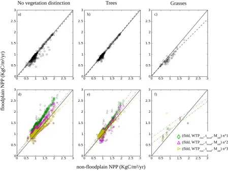
We compared both the simulated grasses/trees contribu-tion to total vegetacontribu-tion and the simulated-floodplain NPP against observations to evaluate whether our modifications capture the floodplain vs. non-floodplain patterns well.
Besides floodplain extent, GLC2000 was used for evaluat-ing the LPX-simulated fractional vegetation cover of flood-plain grasses, floodflood-plain trees, non-floodflood-plain grasses and non-floodplain trees (see Sect. 2.3). For this purpose, the LPX floodplain tree cover was compared to the sum of all the GLC2000 classes listed in Sect. 2.6.1 while “Periodi-cally flooded savannah” was used to evaluate the fraction of flooded grasses in LPX. All other natural tree and grass classes were used to evaluate the non-floodplain grass and tree fractions in LPX at 0.5◦resolution. For LPX, vegetation cover is calculated by summing the FPCs of the PFTs to be compared.
Floodplain NPP was evaluated against the MODerate Res-olution Imaging Spectroradiometer (MODIS)-derived NPP. We made use of GLC2000 to identify the location of flood-plain ecosystems, extracting the NPP of floodflood-plain ecosys-tems only. This approach assumes that, at a 0.5◦
resolu-tion, the differences in NPP between the floodplain and non-floodplain LUs are explained by the flooding conditions. MODIS-NPP was obtained from the Numerical Terrady-namic Simulation Group (NTSG) (Zhao and Running, 2010; Zhao et al., 2005) (http://www.ntsg.umt.edu). We regridded MODIS-derived NPP to the GLC2000 grid. Then, for each
grid cell at LPX resolution, NPP was estimated for differ-ent ecosystem types (floodplain and non-floodplain) as well as for the two vegetation meta-classes (grasses and trees) in these ecosystems. To do so, the GLC2000 maps were used to identify the ecosystem and vegetation type of each MODIS grid cell at GLC2000 resolution. Figure A3 displays the re-sulting NPP maps at GLC2000 resolution, for the quadrant along the main Amazon River defined in Hess et al. (2003). This approach has the following limitations:
– The MODIS data coverage in the Amazon region is strongly limited by cloud cover, which requires gap-filling (Zhao et al., 2005).
– Inconsistencies between MODIS-derived NPP and GLC2000 could occur due to the different resolutions and projections (sinusoidal and regular cylindrical) of the original data sets.
– In MODIS, no NPP values are provided for grid cells corresponding to water bodies, which are set to zero. Note that this mainly concerns the main stem of rivers and lakes, rather than the floodplains themselves. By changing the resolution of the MODIS-derived NPP maps, the missing values influence partially overlap-ping grid cells. This “contamination” is likely to be larger for floodplain than non-floodplain ecosystems, as they are closer to water bodies. This introduces some underestimation of floodplain NPP, but given the overall uncertainty of the approach this is still consid-ered acceptable.
solids (sand) and thus, lower fertility (cf. the Fig. 1 of Junk et al., 2011). This difference in fertility is related to a differ-ence in phosphorus supply (Arago et al., 2009). This leads to differences in vegetation cover (e.g., Belger et al. (2010) and see Sect. 4) and productivity between varzeas and igapos along a west to east gradient (e.g., Gloor et al., 2012). For in-stance, the diameter-increment growth rates of trees are up to two-thirds lower in igapos than those found in varzeas forests (Schöngart et al., 2010).
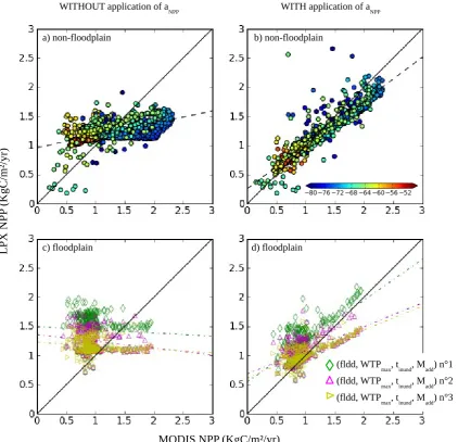
Only recently, LSMs started to include phosphorus dy-namics (Goll et al., 2012). This is not yet the case for the LPX model, which may influence the comparison between the MODIS and LPX-derived NPP of Amazon floodplains. The influence of a neglect of phosphorus dynamics and other shortcomings in the LPX-simulated floodplain NPP is quan-tified by the following ratio:
aNPP(g)= NPPMODISnon−flood(g)/NPPnonLPX−flood(g), (6)
which has been computed for each grid cellgusing the mean annual non-floodplain NPP over the 2000–2009 period. To evaluate the sensitivity of LPX-simulated CH4fluxes to
un-certainties in NPP (i.e., anpp), a second set of simulations
were performed (see Table 1) in which the LPX-computed NPPs for both floodplain and non-floodplain LUs were cor-rected usingaNPP. The scaling factors were applied in LPX
at each time step and for all years from the beginning of the spin-up.
2.6.3 CH4emissions
For the estimation of CH4emissions, LPX simulations were
performed at two spatial scales: the site scale and the Ama-zon Basin scale. LPX-simulated CH4 flux densities and
CH4emissions were compared to available information from
observations at different sites and to results of bottom-up models participating in the WETCHIMP intercomparison (Melton et al., 2013; Wania et al., 2013).
Simulations at individual sites
LPX simulations were performed for five grid cells in the Amazon Basin, where measurements of floodplain CH4flux
densities are available, using the same simulation set-up as discussed in Sect. 2.6.2. Only a few studies report measure-ments from floodplains in this region of the world. All these sites were used for sensitivity analysis and model evaluation. Table 2 gives the main characteristics of each site, including its coordinates, the period of measurements, some technical information about the measurements, as well as vegetation cover at the sampled locations. Among the sites, three are lo-cated in the Negro River floodplain (sites 1, 2 and 3; Belger et al., 2010) and two other sites (site 4, Wassman et al., 1992, and site 5, Bartlett et al., 1988) are located in the central Amazon about 80 km from Manaus. At all sites, measure-ments were performed using flux chambers, funnels and/or
through determination of gas concentration in air and water. Thus, they are representative of a very small spatial scale (the typical chamber area is 0.2 m2).
All sites classify as a floodplain, despite the fact that some are referred to as “floodplain lake” or “lake” in the literature. For example, Marani and Alvalá (2007) (Supp. Site 2) define a “lake” as a permanently flooded area. Usually, measure-ments of CH4flux densities are given for different vegetation
cover (emergent grasses, floating macrophytes, shrubs or for-est) as well as for non-vegetated spots (i.e., open water). All selected five sites include information about CH4 flux
den-sities for at least one vegetated spot. No information about the grass cover (emergent or floating) of the measured plots is available for any of the sites.
In addition, LPX simulations were performed for three ad-ditional sites (cf. the last three lines of Table 2). These sites are used in Sect. 4 to evaluate the ability of our modified LPX version to simulate emission from open-water bodies and emissions outside of the Amazon Basin.
All simulations were compared to observation for those years for which measurements are available (Table 2). CH4
fluxes are evaluated on annual or sub-annual timescales. A sensitivity analysis is performed using six different settings, including an “optimal” simulation (Table 3). Each of the set-tings was compared to the site observations. The simulations mainly vary in vegetation cover, flooding depth and the appli-cation of the NPP scaling factor (aNPP). The first three
simu-lations were performed for the three parameter combinations defined in Table 1. Vegetation was either computed by LPX or prescribed through modifications of WTPmax,tinund and
Madd. To prescribe grasses,Maddwas set to 1. To prescribe
trees at their maximum cover (95 % of the grid cell), WTPmax
andtinundof trees are set equal to the values of flood-tolerant
grasses andMaddwas set to 0. Note, however, that this
strat-egy slightly modifies the inundation stress value. Available information about the observed flood level on site was used to prescribe the flood level in LPX for simulations 2–7 (see Fig. A4). The “optimal” simulation uses conditions that are as close as possible to reality. These conditions vary among sites as described in Table 4.
The “optimal” simulations for sites 1 and 2 include a mod-ification in the root profile and soil porosity according to Bel-ger et al. (2010). For sites 4 and 5, the “optimal” simulation aims at evaluating the sensitivity of the simulated CH4flux
densities to some floating macrophyte properties, namely a suppression of the transport by plants and the fraction of NPP going to exudates set to 0.
Simulations for the Amazon Basin
The set-up of simulations performed for the Amazon Basin is summarized in Table 5. The simulations mainly differ in vegetation characteristics (WTPmax,tinundandMadd), the
pa-rameterization of flooding depth (flddproduct, flddredist), the
Table 2. Description of sites used for sensitivity analysis and CH4flux density evaluation. The three Supp. Sites will be used to discuss the ability of the here-developed LPX version to simulate open-water emissions and floodplain emissions outside of the Amazon Basin. Blank cells mean that no information is available and SFC refers to “static floating chamber”.
Site no.
Name Reference(s) Coordi-nates
Brief description Period (and frequency) of measurements Methods of measurements Technique to separate ebullition and diffusion Vegetation covering of spots Information about flood level
1 Cuini Belger et al. (2011)
0◦690S, 63◦570W
interfluvial wetland in the Negro River basin
monthly during the year 2005
SFC and inver-ted tunnels when habitats were flooded (as well as terrestrial chambers when the environment was unflooded); measures of CH4 concentration in water
inverted funnels
→ebullition; static floating chambers
→diffusion; diffu-sive fluxes also esti-mated using Fick’s law and measures of CH4 concentra-tion in water
open water, emergent grasses, shrubs
permanently flooded; no more than 0.6 m deep
2 Itu 0◦290S,
63◦450W
open water, emergent grasses, shrubs, palms
dried several months per year; up to 1.3 m
3 Araca 0◦190N,
63◦210W
open water, emergent grasses, shrubs, forests
dried several months per year; up to 0.8 m deep
4 Isla Marchan-taria
Wassman et al. (1992)
3◦130S, 59◦550W
a “floodplain lake” located on an island in the Amazon main channel (Varzea) about 15 km south of Manaus
monthly during Apr 1988– Apr 1989
SFC sudden deviation in the increase of mea-sured concentration after closure of the static chamber is attributed to ebulli-tion phenomenon
open water, floating macro-phytes and flooded forest
one value per month (see Fig. A4) but varies among the sites into the flood-plain lake (“temporarily subaerial” vs. “permanent aquatic” sites) 5 Marrecao/ Pesqueiro/ Cabaliana/ Lago Colado
Bartlett et al. (1988)
3◦150S, 60◦750W
sites closed to Lago Calado (cf. Supp. Site 1)
some days during Jul–Aug 1985
SFC as well as discontinuous measurements using air sampling from the headspace of the same floating chambers
SFC: sudden devi-ation is attributed to ebullition pheno-menon. No distinc-tion in the discon-tinuous measure-ments
floating grass macrophytes; flooded forest
values given for a subset of CH4measurement in two habitats of Cabaliana
Supp. Site 1
Lago Colado
Crill et al. (1988)
3◦150S, 60◦340W
lake of about 6 km2 area in the central Amazon Basin located on the north side of the Solimões River, 80 km upriver from its confluence with the Negro River
Monthly during Jul–Aug 1985
SFC as well as discontinuous measurements using air sampling from the headspace par of the same floating chambers
SFC: sudden devi-ation is attributed to ebullition pheno-menon. No distinc-tion in the discon-tinuous measure-ments
open water dry season; Jul: 8.8 m; Aug: 6.6 m
Engle and Melack, 2000
daily during two periods: 18 Apr–27 May 1987 and 14– 24 Sep 1987
Apr–May: mea-sures of surface water CH4 concen-trations
only diffusive flux estimated through empirical expressions
Apr–May: rising waters
Sep: SFC and mea-sures of surface water CH4 concen-tration
diffusive flux esti-mated through em-pirical expres-sions; ebullition = difference bet-ween estimated diffusive flux and measures with SFC
Sep: falling waters
Supp. Site 2 Spot in Pantanal wetland Marani and Alvala (2007)
19◦190S– 19◦340S, 57◦000W– 57◦030W
two “lakes” (per-manent flooded areas: Medalha and Mirante) and three floodplains (flooded seaso-ally: Arara-Azul, Bau, Sao Joao) in the Pantanal region
five campaigns between Mar 2004 and Mar 2005
SFC sudden deviation in the increase of mea-sured concentration after closure of the static chamber is attributed to ebulli-tion phenomenon
floating macro-phytes and open water
Large variability between the sites of “lake” (perma-nently flooded) and “flood-plains”. Flood depth of more than 2.4 m found in only one site (Medalha lake). We assumed maxi-mum flood depth for others sites close to 1.6 m. Dry conditions in one site (Sao Jao) during December campaign which does not allow any measurements. Supp.
Site 3 Spot in Panama
Keller et al. (1990), Table 1 of Barlett and Harris (1993) and Walter and Heimann (2000)
9◦300N, 79◦960W
swamp and flood forest located in Panama
1986 grasses and
flooded forest
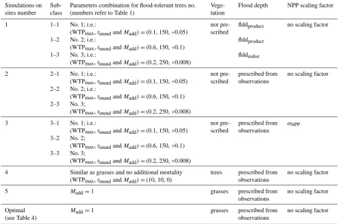
[image:12.595.56.539.104.724.2]Table 3. Set-up for simulations on sites. The parameter combinations (WTPmax,tinund andMadd) refer to Table 1. “Trees”-prescribed
vegetation means that forest occupies 95 % of the grid cell (see text).
Simulations on sites number
Sub-class
Parameters combination for flood-tolerant trees no. (numbers refer to Table 1)
Vege-tation
Flood depth NPP scaling factor
1 1–1 No. 1; i.e.:
(WTPmax,tinundandMadd)=(0.1, 150, +0.05)
not pre-scribed
flddproduct no scaling factor
1–2 No. 2; i.e.:
(WTPmax,tinundandMadd)=(0.6, 150, +0.1)
flddproduct
1–3 No. 3; i.e.:
(WTPmax,tinundandMadd)=(0.2, 250, +0.008)
flddredist
2 2–1 No. 1; i.e.:
(WTPmax,tinundandMadd)=(0.1, 150, +0.05)
not pre-scribed
prescribed from observations
no scaling factor
2–2 No. 2; i.e.:
(WTPmax,tinundandMadd)=(0.6, 150, +0.1)
2–3 No. 3;
(WTPmax,tinundandMadd)=(0.2, 250, +0.008)
3 3–1 No. 1; i.e.:
(WTPmax,tinundandMadd)=(0.1, 150, +0.05)
not pre-scribed
prescribed from observations
aNPP
3–2 No. 2;
(WTPmax,tinundandMadd)=(0.6, 150, +0.1)
3–3 No. 3;
(WTPmax,tinundandMadd)=(0.2, 250, +0.008)
4 Similar as grasses and no additional mortality (WTPmax,tinundandMadd)=(10, 10, 0)
trees prescribed from observations
no scaling factor
5 Madd=1 grasses prescribed from
observations
no scaling factor
Optimal (see Table 4)
Madd=1 grasses prescribed from
observations
no scaling factor
for CH4production/transport. The aim is to estimate the CH4
emission sensitivity to (i) the parameterization of stress and mortality for vegetation (whose major effect is on vegetation distribution), (ii) the flooding depth parameterization, (iii) the introduced modifications in the methanogenesis compu-tation (Eq. 5), (iv) uncertainties in LPX-computed NPP as well as (v) macrophyte properties (last column of Table 5).
Each simulation, except simulation 7, uses the same forc-ing climate data set and spin-up procedure as described in Sect. 2.6.2. Note that each simulation reaches its own equi-librium state after spin-up using its own set of parameters. This strategy differs from Wania et al. (2010), where sen-sitivities were evaluated after perturbing a common equilib-rium state by alternative parameter settings. Our simulation 7 is used to investigate the impact of interannual variation in the wetland extent and thus required a different forcing data set from 1979. While the 1979–2009 climatology of PCR-GLOBWB outputs was used for simulations 1–6 (see Sect. 2.6.2), the year-to-year variability in the floodplain ex-tent given by PCR-GLOBWB was explicitly accounted for to force LPX from 1979 onwards in simulation 7. The modi-fications implemented in LPX to simulate floodplains (inun-dation stress, mortality) lead to different ecosystem
equilib-riums for floodplain and non-floodplain. The implementation of interannual variation in wetland extent from 1979 in simu-lation 7 altered these equilibria. However, the introduced per-turbation was strongly softened in 1993, that is, when the pe-riod of comparison between Simulation 7 and WETCHIMP results started.
The simulation results were compared to estimates of CH4
flux densities representative of large spatial regions. For ex-ample, Bartlett et al. (1990) use a total of 284 flux measure-ments from 42 sampling sites along∼1500 km of the Ama-zon River to compute an average CH4flux density. Average
fluxes are usually given for floating grass mats, flooded for-est, as well as open water. These measurements are gener-ally similar to those described in “Simulations at individual sites” Section. Table 6 provides an overview of the studies that were used, with the corresponding geographical regions and time periods of the measurements. Smith et al. (2000) give a mean CH4flux density for a region along the Orinoco
River, which is used in Section 4 to discuss the ability of LPX to simulate CH4flux densities outside of the Amazon
Table 4. Description of the “optimal” simulation for each site. For each site, the “optimal” simulation has to be compared to the site’s simulation no. 5 (Table 3). According to Wania et al. (2010), the root profile is defined byCrootez/λroot, whereCrootis a normalization
constant to give a total root biomass of 100 % within 2 m depth. Optimal simulation for sites 1 and 2 corresponds to a modification of the
λrootvalue.
Site “Optimal” simulation
1 – Cuini Less deep root profile (λroot=3.2 cm) and increase
in soil porosity (to peatland soil porosity)
2 – Itu Deeper root profile (λroot=85 cm)
3 – Araca No simulation
4 – Isla Marchantaria Tiller porosity = 0 and no exudates for flood-tolerant C4
5 – Marrecao/Pesqueiro/Cabaliana Tiller porosity = 0 and no exudates for flood-tolerant C4
Supp. Site 1 – Lago Colado No simulation
Supp. Site 2 – Spot in Pantanal wetland Tiller porosity = 0 and no exudates for flood-tolerant C4
Supp. Site 3 – Spot in Panama No simulation
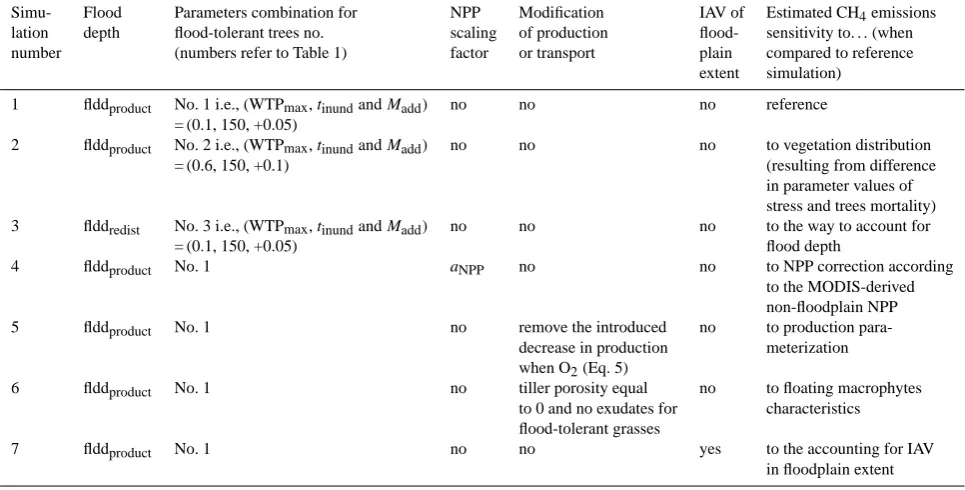
Table 5. Set-up for simulations at Amazon Basin scale.
Simu- Flood Parameters combination for NPP Modification IAV of Estimated CH4emissions
lation depth flood-tolerant trees no. scaling of production flood- sensitivity to. . .(when
number (numbers refer to Table 1) factor or transport plain compared to reference
extent simulation)
1 flddproduct No. 1 i.e., (WTPmax,tinundandMadd) no no no reference
= (0.1, 150, +0.05)
2 flddproduct No. 2 i.e., (WTPmax,tinundandMadd) no no no to vegetation distribution
= (0.6, 150, +0.1) (resulting from difference
in parameter values of stress and trees mortality)
3 flddredist No. 3 i.e., (WTPmax,tinundandMadd) no no no to the way to account for
= (0.1, 150, +0.05) flood depth
4 flddproduct No. 1 aNPP no no to NPP correction according
to the MODIS-derived non-floodplain NPP
5 flddproduct No. 1 no remove the introduced no to production
para-decrease in production meterization
when O2(Eq. 5)
6 flddproduct No. 1 no tiller porosity equal no to floating macrophytes
to 0 and no exudates for characteristics
flood-tolerant grasses
7 flddproduct No. 1 no no yes to the accounting for IAV
in floodplain extent
CH4flux densities are computed for the entire floodplain LU
without distinguishing among PFTs, we classified each grid cell as a “flooded forest” or “flooded grasses” ecosystem us-ing four different criteria (details in Appendix A). In each case, only grid cells where floodplain cover was greater than 5 % of the grid cell were retained.
Finally, the floodplain CH4 emissions were compared to
the outputs of the models participating in the WETCHIMP intercomparison (Melton et al., 2013; Wania et al., 2013). WETCHIMP (Wetland and Wetland CH4Intercomparison of
Models Project) was organized to evaluate our present abil-ity to simulate large-scale wetland characteristics and corre-sponding CH4emissions. In the present study, we use
emis-sion estimates for the Amazon Basin from six WETCHIMP
models (see right panel of Table 7). An overview of the com-putation in the WETCHIMP models of the two components that determine total CH4 emissions (i.e., the CH4 flux
[image:14.595.57.540.275.520.2]Table 6. Available information about CH4flux density at large scale. Geographical areas selected to estimate comparable LPX-computed CH4flux densities are given in the last column. Areas 1 and 2 are in the Amazon Basin, while the last area (Supp. Site 1) is located in
the Orinoco Basin. Despite some differences in the spots used to estimate the mean CH4flux density, we consider that Devol et al. (1988),
Bartlett et al. (1990) and Devol et al. (1990) give information about the same geographical area.
Area number
Reference Area of measurements Period of measurements Area used in LPX to compute the mean CH4flux density
1 Devol et al. (1988) (corrected by Bartlett et al., 1990)
“fringing” floodplains along∼1700 km of the Amazon River main stem; between “Vargem Grande” and Obidos
Jul–Aug 1985 (early falling water period of the flood cycle)
quadrate defined by: latitude: [5◦S:1.5◦S] longitude: [70◦W:55◦W]
Bartlett et al. (1990) Apr–May 1987 (wet season
as river water levels were high and rising)
quadrate defined by: latitude: [5◦S:1.5◦S] longitude: [70◦W:55◦W]
Devol et al. (1990) Nov–Dec 1988 (low water
period of the annual flood cycle)
quadrate defined by: latitude: [5◦S:1.5◦S] longitude: [70◦W:55◦W]
2 eight lakes near Manaus
(03◦060S; 60◦010W)
May 1987–Sep 1988 quadrate defined by: latitude: [3.5◦S:2.5◦S] longitude: [60.5◦W:59.5◦W]
Supp. Area 1
Smith et al. (2000) “fringing” floodplains along a 600 km-reach of the Orinoco main stem and the upper delta
Jul 1991–Sep 1992 quadrate defined by: latitude: [7◦N:10◦N] longitude: [66◦W:60.5◦W]
in the Amazon Basin, the spatial distribution as well as the temporal variability (both the seasonal and year-to-year vari-ability) of the two above-cited CH4emissions components.
Given the uncertainty in the Amazon floodplain extent and the high estimates thereof by PCR-GLOBWB, as compared to GLC2000 (see Sect. 3.1), the emission sensitivity to flood-plain extent was evaluated. To do so, we only retained grid cells where the GLC2000 flooded vegetation fraction was larger than 2 %. For these grid cells, PCR-GLOBWB out-puts were used to provide both floodplain extent and flooding depth.
3 Results
3.1 Floodplain extents
Around 6.8 % of South America is covered by floodplain ac-cording to PCR-GLOBWB, against only 3.7 % in GLC2000 (Fig. 1). Outside of the Amazon Basin, GLC2000 and PCR-GLOBWB agree relatively well, such as for floodplains in the Pantanal and along the Parana River. However, the largest differences are found within the Amazon Basin, in partic-ular in the south of the basin and along the Amazon River itself: 4.1 and 12.2 % of the Amazon Basin are covered by floodplains for GLC2000 and PCR-GLOBW, respectively. If only grid cells where the GLC2000 flooded vegetation
frac-tion is larger than 2 % are retained, fldfmeanreaches 6.7 %, in
other words, a value much closer to the GLC2000 estimates. This means that the mismatch between PCR-GLOBWB and GLC2000 at 0.5◦resolution is mainly explained by the pres-ence of additional (small) floodplains in PCR-GLOBWB, in-stead of a large disagreement in the extent of floodplains that are accounted for in both estimates.
This difference may be explained in part by the fact that fldfmean is only based on hydrological processes, whereas
GLC2000 represents land fractions where the floodplain veg-etation is dominant. fldfmeanmight be interpreted as the