www.geosci-model-dev.net/7/2411/2014/ doi:10.5194/gmd-7-2411-2014
© Author(s) 2014. CC Attribution 3.0 License.
Improved simulation of fire–vegetation interactions in the
Land surface Processes and eXchanges
dynamic global vegetation model (LPX-Mv1)
D. I. Kelley1, S. P. Harrison1,2, and I. C. Prentice1,3
1Department of Biological Sciences, Macquarie University, North Ryde, NSW 2109, Australia
2Geography & Environmental Sciences, School of Archaeology, Geography and Environmental Sciences (SAGES),
University of Reading, Whiteknights, Reading, RG6 6AH, UK
3AXA Chair of Biosphere and Climate Impacts, Grantham Institute for Climate Change and Department of Life Sciences,
Imperial College, Silwood Park Campus, Ascot SL5 7PY, UK
Correspondence to: D. I. Kelley ([email protected])
Received: 30 October 2013 – Published in Geosci. Model Dev. Discuss.: 23 January 2014 Revised: 16 July 2014 – Accepted: 25 July 2014 – Published: 16 October 2014
Abstract. The Land surface Processes and eXchanges (LPX) model is a fire-enabled dynamic global vegetation model that performs well globally but has problems representing fire regimes and vegetative mix in savannas. Here we fo-cus on improving the fire module. To improve the represen-tation of ignitions, we introduced a treatment of lightning that allows the fraction of ground strikes to vary spatially and seasonally, realistically partitions strike distribution be-tween wet and dry days, and varies the number of dry days with strikes. Fuel availability and moisture content were im-proved by implementing decomposition rates specific to indi-vidual plant functional types and litter classes, and litter dry-ing rates driven by atmospheric water content. To improve water extraction by grasses, we use realistic plant-specific treatments of deep roots. To improve fire responses, we in-troduced adaptive bark thickness and post-fire resprouting for tropical and temperate broadleaf trees. All improvements are based on extensive analyses of relevant observational data sets. We test model performance for Australia, first evalu-ating parameterisations separately and then measuring over-all behaviour against standard benchmarks. Changes to the lightning parameterisation produce a more realistic simula-tion of fires in southeastern and central Australia. Implemen-tation of PFT-specific decomposition rates enhances perfor-mance in central Australia. Changes in fuel drying improve fire in northern Australia, while changes in rooting depth produce a more realistic simulation of fuel availability and
structure in central and northern Australia. The introduction of adaptive bark thickness and resprouting produces more re-alistic fire regimes in Australian savannas. We also show that the model simulates biomass recovery rates consistent with observations from several different regions of the world char-acterised by resprouting vegetation. The new model (LPX-Mv1) produces an improved simulation of observed vegeta-tion composivegeta-tion and mean annual burnt area, by 33 and 18 % respectively compared to LPX.
1 Introduction
models, have been shown to be unrealistic (Prentice et al., 2011; Bistinas et al., 2014). LPX realistically simulates fire and vegetation cover globally but performs relatively poorly in grassland and savanna ecosystems (Kelley et al., 2013) – areas where fire is particularly important for maintaining vegetation diversity and ecosystem structure (e.g. Williams et al., 2002; Lehmann et al., 2008; Biganzoli et al., 2009). Specifically:
– LPX produces sharp boundaries between areas of high burning and no burning in tropical and temperate regions. These sharp fire boundaries produce sharp boundaries between grasslands and closed-canopy forests. The unrealistically high fire-induced tree mor-tality prevents the development of vegetation charac-terised by varying mixtures of tree and grass plant func-tional types (PFTs) that are characteristic of more open forests, savannas and woodlands.
– LPX simulates too little fire in areas of high but seasonal rainfall because fuel takes an unrealistically long time to dry, and because LPX fails to produce open woody vegetation in these areas.
– In arid areas, where fire is limited by fuel availability, LPX simulates too much net primary production (NPP) resulting in unrealistically high fuel loads and generat-ing more fire than observed.
To address these shortcomings in the version of LPX run-ning at Macquarie University (here termed LPX-M), we re-parameterised lightning ignitions, fuel moisture, fuel de-composition, plant adaptations to arid conditions via rooting depth, and woody plant resistance to fire through bark thick-ness. In each case, the new parameterisation was developed based on extensive data analysis. We tested each parameter-isation separately, and then all parameterparameter-isations combined, using a comprehensive benchmarking system (Kelley et al., 2013) which assesses model performance against observa-tions of key vegetation and fire processes. We then included a new treatment of woody plant recovery after fire through resprouting – a behavioural trait that increases post-fire com-petitiveness compared to non-resprouters in fire-prone areas (Clarke et al., 2013) and thus affects the speed of ecosys-tem recovery with major implications for the carbon cy-cle – and tested the impact of introducing this new com-ponent on model performance. In this paper, we begin by describing the basic fire parameterisations in LPX (Sect. 2) and then go on to explain how these parameterisations were changed in LPX-Mv1 (Sect. 3) before evaluating whether these new data-derived parameterisations improve the sim-ulation of vegetation patterns and fire regimes (Sect. 4).
2 LPX model description
LPX is a plant-functional-type (PFT)-based model. Nine PFTs are distinguished by a combination of life form (tree, grass) and leaf type (broad, needle), phenology (evergreen, deciduous) and climate range (tropical, temperate, boreal) for trees and photosynthetic pathway (C3, C4) for grasses. PFTs
are represented by a set of parameters. Each PFT that oc-curs within a grid cell is represented by an “average” plant, and ecosystem-level behaviour is calculated by multiplying the simulated properties of this average plant by the simu-lated number of individuals in the PFT in that grid cell. PFT-specific properties (e.g. establishment, mortality and growth) are updated annually, but water and carbon-exchange pro-cesses are simulated on shorter time steps.
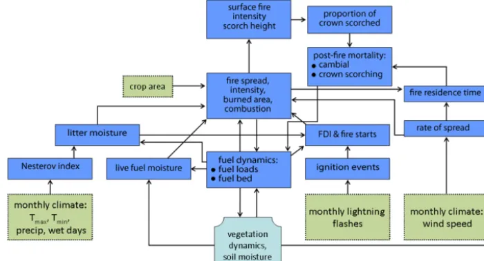
LPX incorporates a process-based fire scheme (Fig. 1) run on a daily time step (Prentice et al., 2011). The LPX fire scheme is modified from the Spread and Ignitions FIRE model (SPITFIRE; Thonicke et al., 2010). In this section, we describe those aspects of the LPX fire model that appear to contribute to poor simulation of fire regimes in Australia (and likely other semiarid regions) and which we have re-examined and re-parameterised on the basis of data analy-ses (see Sect. 3). Ignition rates are derived from a monthly lightning climatology, interpolated to the daily time step. The number of lighting strikes that reach the ground (cloud to ground; CG) is specified as 20 % of the total number of strikes (Thonicke et al., 2010). The CG lightning is split into dry (CGdry) and wet strikes based on the fraction of wet days
in the month (Pwet):
CGdry=CG·(1−Pwetβ ), (1)
whereβ is a parameter tuned to 0.00001. “Wet” lightning is not considered to be an ignition source (Prentice et al., 2011). Lightning is finally scaled down by 85 % to allow for dis-continuous current strikes. Numerical precision limits of the compiled code means the function described by Eq. (1) effec-tively removes all strikes in months with more than two wet days in LPX. Monthly “dry” lightning is distributed evenly across all dry days.
Fuel loads are generated from litter production and de-cay using the vegetation dynamics algorithms in LPJ (Lund– Potsdam–Jena; Sitch et al., 2003). LPX does not simulate competition between C3 and C4 grasses explicitly; in grid
cells where C3and C4grasses co-exist, the total NPP is
Figure 1. Description of the structure of the fire component of LPX, reproduced from Prentice et al. (2011). Inputs to the model are identified by green boxes, outputs from the vegetation dynamics component of the model are identified by light blue boxes, and internal processes and exchanges that are explicitly simulated by the fire component of the model are identified by blue boxes. FDI is the Nesterov Fire Danger Index.
Fuel decomposition rate (k) depends on temperature and moisture, and is the same for all PFTs and fuel structure types:
k=k10·g(T )·f (w), (2)
where k10 is a decomposition rate at a reference
tempera-ture of 10◦C, set to 35 % each year;g(T )describes the re-sponse to monthly mean soil temperature (Tsoil, m) described
by Lloyd and Taylor (1994):
g(T )=
e308.56·
1 56.02−
1
Tsoil, m+46.02
, ifTsoil, m≥ −40
0, otherwise,
(3)
andf (w)is the moisture response to the top layer soil water content (w) described by Foley (1995):
f (w)=0.25+0.75·w, (4)
wherewis in fractional water content.
The litter is allocated to four fuel categories based on litter size as described by Thonicke et al. (2010):
– 1 h fuel – which represents leaves and small twigs, is the leaf and herb mass plus 4.5 % of the litter that comes from tree heart- and sapwood.
– 10 h fuel – representing small branches, is 7.5 % of the litter from heart- and sapwood.
– 100 h fuel – large branches, is 21 % of the litter that comes from heart- and sapwood.
– 1000 h fuel – boles and trunks, is the remaining 67 % of the litter that comes from heart- and sapwood.
The hour designation represents the decay rate of fuel moisture, and is equal to the amount of time for the mois-ture of the fuel to become (1−1/exp)=63 % closer to the moisture of its surroundings (Albini, 1976; Anderson et al., 1982).
In LPX, litter drying rate is described by the cumulative Nesterov fire danger index (NI; Nesterov, 1949) as described by Running (1987), and a fuel-specific drying rate param-eter (αxhr; Venevsky et al., 2002) which was tuned to
pro-vide the best results against fire observations (Thonicke et al., 2010). NI is cumulated for each consecutive day with rain-fall≤3 mm, and is calculated using maximum daily temper-ature (Tmax) and an approximation of dew point temperature:
Tdew=Tmin−4, (5)
whereTminis the daily minimum temperature and bothTmin
andTmaxare in degrees Celcius.
Daily precipitation is simulated based on monthly precipi-tation and fractional wet days using a simple weather genera-tor (Gerten et al., 2004), and the diurnal temperature range is calculated from daily maximum and minimum temperature interpolated from monthly data.
Fire spread, intensity and residence time are based on weather conditions and fuel moisture, and calculated using the Rothermel equations (Rothermel, 1972). Fire intensity and residence time influence fire mortality via crown scorch-ing and cambial damage.
and intercept values for each PFT:
BT=a+b·DBH. (6)
The values of a and b can be found in Thonicke et al. (2010).
The probability of mortality from cambial damage (Pm) is
calculated from the fire residence time (τl) and a critical time
till cambial damage (τc) based on bark thickness:
Pm(τ )=
0, if τl
τc≤0.22
0.563·τl
τc−0.125, if 0.22≤
τl
τc ≤2
1, if τl
τc≥2
(7)
and
τc=2.9·BT2, (8)
whereτ is the ratioτl/ τc. Bothτlandτcare in minutes and
BT is in centimetres.
LPX uses a two-layer soil model. The water content of the upper (50 cm) layer is the difference between throughfall (precipitation−interception) and evapotranspiration (ET), and runoff and percolation to the lower soil layer. Water con-tent in the lower 1 m layer is the difference between percola-tion from the upper layer, transpirapercola-tion from deep roots and runoff (Gerten et al., 2004). The upper soil layer responds more rapidly to changes in inputs, whereas the water content of the lower soil layer is generally more stable. The fraction of roots in each soil layer is a PFT-specific parameter.
3 Changes to the LPX-M fire module
Improvements to the LPX-M fire module focussed on re-parameterisation of lightning ignitions, fuel drying rate, fuel decomposition rate, rooting depth, and the introduction of adaptive bark thickness and of resprouting. The improve-ments are based on analyses of large-scale regional and/or global data sets, and are therefore generic. Although we fo-cus on Australia for model evaluation, we have made no at-tempt to tune the new parameterisations using Australian ob-servations.
3.1 Lightning ignitions
Regional studies have shown that the CG proportion of to-tal lightning strikes varies between 0.1 and 50 % of toto-tal strikes. This variability has been related to latitude (Price and Rind, 1993; Pierce, 1970; Prentice and Mackerras, 1977), storm size (Kuleshov and Jayaratne, 2004), total flash count (Boccippio et al., 2001), and topography (Boccippio et al., 2001; de Souza et al., 2009). We compared remotely sensed data on total flash counts (i.e. intercloud, or IC, plus CG) from the Lightning Imaging Sensor (LIS – Christian et al., 1999; Christian, 1999, http://grip.nsstc.nasa.gov/) with the
National Lightning Detection Network Database (NLDN) records of lightning ground-strikes (CG) for the contiguous United States (see http://thunderstorm.vaisala.com/ for infor-mation; Cummins and Murphy, 2009), for each month in 2005 at the 0.5◦resolution of LPX. These analyses were con-fined to south of 35◦N, a limitation imposed by satellite cov-erage of the total strikes (Christian et al., 1999).
The LIS observed each cell for roughly 90 s during each overpass, with 11–21 overpasses each month depending on latitude (Christian et al., 1999), and therefore only represents a sample of the total lightning. Overpasses for each 0.5◦ cell have a time stamp for the start and end of each over-pass, along with detection efficiency and total observation time, which allows for observational blackouts. We scaled the flash count from each overpass for detection efficiency and the ratio of observed to total overpass time. These scaled flash counts were summed for each month, to give monthly recorded total lightning (RL), which includes both cloud to cloud and cloud to ground strikes (i.e. IC+CG).
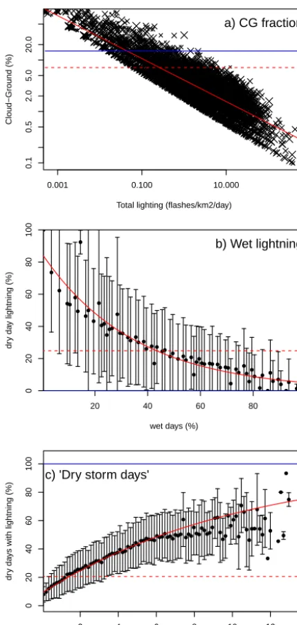
NLDN registered each ground lightning strike separately with a time stamp accurate to 1/1000th of a second, which al-lowed us to calculate the number of ground-registered NLDN strikes for each LIS overpass. This number of ground strikes was then scaled for a universal detection efficiency of 90 % (Boccippio et al., 2001; Cummins and Murphy, 2009), and summed up for the month, to give monthly recorded CG strikes (RG). The CG fraction was taken as RG/RL. Total flash count (L) was calculated by scaling the total ground registered lightning for each month by the CG fraction. The relationship between fractional CG and total lightning was determined using non-linear least squares regression, testing for both power and exponential functions. The best (Fig. 2a) was given by
CG=L·min(1,0.0408·L−0.4180), (9) whereLis in flash km−2day−1. We also tested topography and topographic complexity, calculated from topographic data from WORLDCLIM (Hijmans et al., 2005). These vari-ables were not significantly related to the observed CG frac-tion, and so we have not included them as predictors in the new parameterisation.
We examined the relationship between CG strikes and the daily distribution of precipitation using the Climate Pre-diction Center (CPC) US Unified Precipitation data (Hig-gins and Centre, 2000; Hig(Hig-gins et al., 1996) provided by the NOAA/OAR/ESRL PSD (Physical Sciences Division), Boulder, Colorado, USA (http://www.esrl.noaa.gov/psd/). Days are classified as dry if there was zero precipitation. We used data for every month of 2005, this time covering the whole of the contiguous United States. We used gener-alised linear modelling (GLM; Hastie and Pregibon, 1992) to compare CGdry to Pwet and monthly precipitation from
0.001 0.100 10.000 0.1 0.5 2.0 5.0 20.0
Total lighting (flashes/km2/day)
Cloud−Ground (%)
a) CG fraction
● ● ● ●● ● ● ● ● ● ● ● ●● ● ●● ● ●● ●●● ● ● ●● ● ● ●● ●●●● ●● ● ●●●● ●● ● ● ●● ● ● ● ● ● ● ● ● ● ● ● ● ● ●● ● ● ● ●
20 40 60 80
0 20 40 60 80 100
wet days (%)
dr
y da
y lightning (%)
b) Wet lightning
●● ●●●●● ●● ●●●●●● ●●●●●●●● ●●●●●● ●●●●●● ●●●●●●●●●●● ● ●●●●●● ● ●●● ● ●●●●●● ● ●● ● ●● ● ● ●● ● ● ● ● ● ●● ● ● ● ● ● ● ● ● ● ● ● ● ●
2 4 6 8 10 12
0 20 40 60 80 100
Monthly dry CG lightning strikes (strikes/km2/day)
dr
y da
ys with lightning (%)
c) 'Dry storm days'
Figure 2. Observed relationships between (a) total and cloud-to-ground lightning flashes, (b) the percentage of dry lightning with respect to the number of wet days per month, and (c) percent-age of dry days with lightning with respect to monthly dry light-ning strikes. These analyses are based on the LIS remotely sensed data set (Christian et al., 1999; Christian, 1999) and NLDN ground observation of lightning strikes (Cummins and Murphy, 2009) for North America. The red line shows the best fit used by LPX-Mv1, the red dotted line shows the mean of the observations, and the blue line shows the relationship used in LPX. To aid visualisation, ob-servations were binned every 1 % (b) or 0.1 strikes (c) along thex
axis, with the dots showing the mean of each bin and the error bars showing the standard deviations.
(Harris et al., 2013).Pwetfrom both CPC and CRU were the
best and only significant predictors. Using CPC for consis-tency, the best relationship for CGdry(Fig. 2b) was
CGdry=0.85033·CG·e−2.835·Pwet, (10)
where CGdryis the number of strikes on days with zero
pre-cipitation, andPwet is the amount of precipitation on days
with rain. We determined a new parameter for the fraction of dry days with lightning strikes (“dry storm days”) by compar-ing the fraction of dry days in CPC when lightncompar-ing occurred (Pdry, lightn) with CGdry calculated in Eq. (10) (Fig. 2c). The
analysis was performed using the same spatial domain as the analysis of CGdry. The best relationship with the least
squared residuals (Fig. 2c) was
Pdry lightn=1−
1
1.099·(CGdry+1)94 678.69
. (11)
The results of these analyses were used in the new pa-rameterisation of lightning in LPX-Mv1. IC lightning was removed by applying Eq. (9), where L is taken from the monthly lightning climatology inputs. Wet lightning was re-moved from the remaining CG strikes by applying Eq. (10). A sensitivity test including lightning on wet days shows that such ignitions have little impact or degrade the simulation of burnt area (see Supplement). The remaining CGdry was
distributed evenly onto the number of dry days defined by Eq. (11). The dry lightning days were selected randomly from the days without precipitation as determined by the weather generator (Gerten et al., 2004). Polarity affects the duration of lightning pulses, with negative polarity more likely to produce discontinuous pulses that are insufficient to raise the temperature to ignition point. This discontinuous current lightning was removed at the same constant rate as in LPX because there are no data sets that would allow analyses on which to base a re-parameterisation.
3.2 Fuel drying
The formulation of fuel drying in LPX results in drying times that are too slow in most tropical and temperate regions. Un-der stable and dry weather conditions with a Tmaxof 30◦C
andTdew of 0◦C, for example, 1 h fuel in LPX would take
25 h to lose 63 % of its moisture, 10 h fuel would take roughly 20 days, 100 h fuel would take 2 months, and 1000 h fuel would take 3 yr. The approximation ofTdewused in LPX has
been shown to be too high in arid and semiarid areas, and during dry periods in seasonal climates (Friend, 1998; Run-ning, 1987), which also contributes to slower-than-expected drying. Additionally, given that the moisture content is calcu-lated cumulatively, a sequence of days with<3 mm of rain could result in complete drying of fuel, no matter what the moisture content of the air.
In order to improve this formulation, we replace the de-scription of fuel moisture content in LPX with one based on the moisture content of the air. As fuel types are distin-guished by the time it takes for fuel to come into equilib-rium with the surroundings, this new formulation is consis-tent with the definition of fuel types. Fuel moisture decays towards an “equilibrium moisture content” (meq) at a rate
that matches the definition of the fuel class (i.e, 1 h fuel takes 1/24th of a day to become 63 % closer tomeq):
mx,d=
meq
100+
mx,d−1−
meq
100
·e−24/x, (12)
wheremx,dis the daily moisture content of fuel size in each
drying-time class (x) with a moisture decay rate of 24/x; and mx,d−1is the moisture content on the previous day.
There are several choices of fuel equilibrium models that could be used for meq, with variation in the magnitude of
the meq response to relative humidity (HR), particularly at
extremes (i.e HR→0, 100 %), and the potential for
oppo-site responses to temperature depending on weather condi-tions (Sharples et al., 2009; Viney, 1991). Viney (1991) at-tributed this variation to the choice of fuel type for which each model was calibrated. We chose the model described by Van Wagner and Pickett (1985) formeqas it has been
cal-ibrated against multiple fuel types (Van Wagner, 1972) and is designed to be more accurate at both high and low HR
(Sharples et al., 2009; Viney, 1991):
meq=
(
meq,1+meq,2+meq,3, if Prd≤3 mm
100, otherwise, (13)
where
meq,1=0.942·(HR0.679), (14)
meq,2=0.000499·e0.1·HR, (15)
meq,3=0.18·(21.1−Tmax)·(1−e−0.115·HR). (16)
HR is calculated using the August–Roche–Magnus
ap-proximation (Lawrence, 2005), which has been shown to be
accurate forTdewof between 0 and 50◦C and forTmax
be-tween 0 and 60◦C (Lawrence, 2005):
HR=100·
e17.271·Tdew/(237.7+Tdew)
e17.271·Tmax/(237.7+Tmax). (17)
We use a new formulation forTdewderived from
informa-tion from 20 weather stainforma-tions across the United States (Kim-ball et al., 1997):
Tdew,k=
Tmin,k·(−0.127+1.121·WEF+0.0006·1T ), (18)
whereTdew,k is the daily dew point temperature in Kelvin; 1T is the difference between dailyTmaxandTmin, andWEF
is given by WEF=
(1.003−1.444·EF+12.312·EF2−32.766·EF3), (19) where EF is the ratio of daily potential evapotranspiration (PETd) – calculated as described in Gerten et al. (2004) –
and annual precipitation (Pra):
EF=PETd/Pra. (20)
Kimball et al. (1997) showed that this approximation of Tdew improved the correlation with Tdew measurements by
20 % when tested against 32 independent weather stations, withTdew showing differences of up to 20◦C in semiarid
and arid climates. The more conventional assumption that Tdew=Tmin−4 would thus result in higher dew-point
tem-peratures and slower fuel-drying rates. Although we have re-placed the formulation of fuel-drying rate, including the for-mulation ofTdew, we continue to use the NI to describe the
likelihood of an ignition starting a fire in LPX-Mv1. 3.3 Fuel decomposition
Fuel decomposition rates vary with the size and type of ma-terial (Cornwell et al., 2008, 2009; Weedon et al., 2009; Chave et al., 2009). Brovkin et al. (2012) analysed decompo-sition rates derived from the TRY plant trait database (Kattge et al., 2011, http://www.try-db.org/TryWeb/About.php) and showed that there was an order of magnitude difference in the decomposition rates of wood and leaf/grass litter. Thus, grass decomposes at an average rate of 94 % per year, while wood decomposes at a rate of 5.7 % per year. The rate of both leaf and wood decomposition varies between PFTs to a lesser extent than between wood and grass, although the variation is still significant (Brovkin et al., 2012), with leaf decom-position ranging between 76 and 120 %, and wood between 3.9 and 10.4 % per year (Table 1). Brovkin et al. (2012) also showed that the decomposition rates of woody material are not moisture dependent.
We have implemented the PFT-specific relationships found by Brovkin et al. (2012), for woody (k10,woodfor 10–
Table 1. PFT-specific values used in LPX-Mv1. TBE denotes tropical broadleaf evergreen tree, TBD denotes tropical broadleaf deciduous tree, tBE denotes temperate broadleaf evergreen tree, and tBD temperate broadleaf deciduous tree. Values for RS variants of each of these PFTs are given in brackets. If no resprouting value is given then the resprouting PFT takes the normal PFT value. tNE denotes temperate needleleaf evergreen; BNE denotes boreal needleleaf evergreen; BBD denotes boreal broadleaf deciduous; C3denotes grasses using the C3 photosynthetic pathway; and C4denotes grasses using the C4photosynthetic pathway. BT pari is the bark thickness parameter used
in Eqs. (25) and (26);k10,leaf andk10,woodare the reference litter decomposition rates of leaf and grass used in Eq. (2); andQ10is the parameter describing woody litter decomposition rate changes with temperature in Eq. (21).
TBE TBD tNE tBE tBD BNE BBD C3 C4 Source
Fraction of roots in upper soil layer
0.80 0.70 0.85 0.80 0.80 0.85 0.80 0.90 0.85 Sect. 3.4; Table 2; Fig. 3
BT parlower 0.00395 0.00463 0.00609 0.0125 0.00617 0.0158 0.00875 N/A N/A
(0.0292) (0.0109) (0.0286) (0.0106) Sect. 3.5;
BT parmid0 0.0167 0.0194 0.0257 0.0302 0.0230 0.0261 0.0316 N/A N/A Table S1;
(0.0629) (0.0568) (0.0586) (0.0343) Fig. 4
BT parupper 0.0399 0.0571 0.0576 0.0909 0.0559 0.0529 0.112 N/A N/A (0.183) (0.188) (0.156) (0.106)
k10,leaf 0.93 1.17 0.70 0.86 0.95 0.78 0.94 1.20 0.97 Sect. 3.3;
k10,wood 0.039 0.039 0.041 0.104 0.104 0.041 0.104 N/A N/A Brovkin et al. (2012)
Q10 2.75 2.75 1.97 1.37 1.37 1.97 1.37 N/A N/A
Table 1) litters. We use a relationship between decomposi-tion and temperature for woody fuel that removes the soil moisture dependence in LPX:
kwood=k10,wood·Q
(Tm,soil−10)/10
10 . (21)
Q10is the PFT-specific temperature response of wood
de-composition described in Table 1 andk10,woodis the
decom-position rate at a reference temperature of 10◦C. Leaf
de-composition still follows Eq. (2). 3.4 Rooting depth
There are inconsistencies in the values used in LPX for the fraction of deep roots specified for each PFT. For example, the fraction of deep roots specified for C4grasses (20 %) is
greater than the fraction specified for tropical broadleaf ever-green trees (15 %), even though trees have deeper roots than grasses (Schenk and Jackson, 2005). Additionally, bench-marking against arid grassland and desert litter production shows that simulated fine-litter production is roughly 250 % greater than observations. Having a high proportion of deep roots allows plants to survive more arid conditions, thanks to a more stable water supply in deep soil.
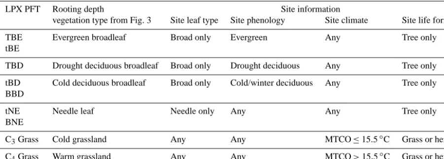
We re-examined the PFT-specific values assigned to root-ing fraction usroot-ing site-based data for the cumulative rootroot-ing fraction depth from Schenk and Jackson (2002a, b, 2005). In the original publications, life form, leaf type, leaf phenology and the cause of leaf fall (i.e. cold or drought) were recorded for each site. This allowed us to classify sites into LPX PFTs as shown in Table 2. The original data source does not dis-tinguish different types of grassland. We therefore separated these sites into warm (C4 dominated) and cool (C3
domi-nated) grasslands depending on their location and climate. Sites were classified as warm grasslands if they occurred in
locations where the mean temperature of the coldest month (MTCO) was>15.5◦C and to cool grasslands where MTCO was≤15.5◦C as in Harrison et al. (2010). MTCO for each site was based on average conditions for 1970–2000 derived from the CRU TS3.1 data set (Harris et al., 2013).
The rooting-depth data set gives the cumulative fraction depth of 50 (D50) and 95 % (D95) of the roots at a site. These
were used to calculate the cumulative root fraction at 50 cm (i.e the fraction in the upper soil layer):
R50 cm=1/(1+(0.5/D50c )), (22)
where
c= log 0.5/0.95
logD95/D50
. (23)
We derived Eqs. (22) and (23) by re-arranging Eq. (1) in Schenk and Jackson (2002b).
The PFT-specific (Fig. 3) fraction of deep roots (DRpft) is
then implemented as
DRpft=1−mean(R50 cm,pft). (24)
See Table 1 for new parameter values. 3.5 Bark thickness
Table 2. Translation between LPX PFTs and the vegetation trait information available for sites which were used to provide rooting depths.
LPX PFT Rooting depth Site information
vegetation type from Fig. 3 Site leaf type Site phenology Site climate Site life form
TBE Evergreen broadleaf Broad only Evergreen Any Tree only
tBE
TBD Drought deciduous broadleaf Broad only Drought deciduous Any Tree only
tBD Cold deciduous broadleaf Broad only Cold/winter deciduous Any Tree only
BBD
tNE Needle leaf Needle only Any Any Tree only
BNE
C3Grass Cold grassland Any Any MTCO≤15.5◦C Grass or herb
C4Grass Warm grassland Any Any MTCO>15.5◦C Grass or herb
dro
ug
ht
d
eci
du
ou
s
b
ro
ad
le
af
co
ld
d
eci
du
ou
s
b
ro
ad
le
af
eve
rg
re
en
b
ro
ad
le
af
needleleaf
tro
pi
ca
l
g
ra
ss
te
mp
era
te
g
ra
ss
40
50
60
70
80
90
100
%
ro
ot
s
in
to
p
50
cm
of
so
il
Figure 3. Proportion of roots in the upper 50 cm of the soil by PFT. The data were derived from Schenk and Jackson (2002a, 2005) and reclassified into the PFT recognised by LPX as shown in Table 2.
et al., 2004; Cochrane, 2003; Lawes et al., 2011a). Thus, at an ecosystem level, bark thickness is an adaptive trait.
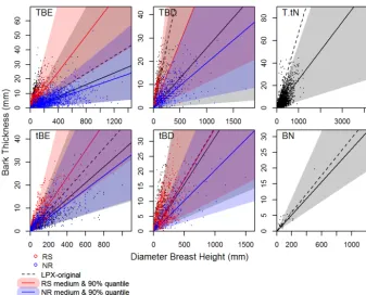
We assess the relationship between bark thickness and stem diameter based on 13 297 measurements from 1364 species (see Supplement for information on the stud-ies these were obtained from). The specstud-ies were classified into PFTs based on their leaf type, phenology and climate range (Table S1 in the Supplement); in cases where this was not provided by the original data contributors, we used in-formation from trait databases, floras and the literature (e.g Kauffman, 1991; Greene et al., 1999; Bellingham and Spar-row, 2000; Williams, 2000; Bond and Midgley, 2001; Del Tredici, 2001; Pausas et al., 2004; Paula et al., 2009; Lunt et al., 2011). The climate range was based on the overall range of the species, not derived from the climate of the sites.
For each PFT, we calculated the best fit and the 5–95 % range (Koenker, 2013, Fig. 4) using the simple linear rela-tionship:
BTi=pari·DBH, (25)
whereiis either the best fit (mid) or in the 5–95 % (lower– upper) range. Values for pari are given in Table 1.
We define a probability distribution of bark thicknesses for each PFT using a triangular relationship defined by the 5 and 95 % limits of the observations (Fig. 4):
T (BT)=
0, if BT≤BTlower
T1(BT), if BTlower≤BT≤BTmid
T2(BT), if BTmid≤BT≤BTupper
0, if BT≥BTupper
, (26)
where BTlower/BTupper/BTmidare the upper/lower/mid range
of BT for a given DBH, calculated using Eq. (25), with pari values in Table 1; and
T1(BT)=
2·(BT−BTlower)
(BTupper−BTlower)·(BTmid−BTlower)
, (27)
T2(BT)=
2·(BTupper−BT)
(BTupper−BTlower)·(BTlower−BTmid)
. (28)
Figure 4. BT vs. DBH for each LPX PFT. Red dots show data used to constrain BT parameters in Table 1 for RS PFTs in LPX-Mv1-rs; blue dots show data from NR PFTs in LPX-Mv1-rs. Red, blue and grey dots are used to distinguish the PFTs in LPX-Mv1-nr. Red and blue lines show best fit lines. Red/blue shaded areas show 90 % quantile ranges. Black line/shaded area shows the best fit and 90 % range for all points. The black dotted line is the relationship used in LPX-M.
The average bark thickness of trees surviving fire is depen-dent on the current state ofT (BT)andPmgiven in Eq. (7),
and is calculated by solving the following integrals: BTmean=
N∗·R BTupper
BTlower BT·(1−Pm(τ ))·T (BT)dBT.
N , (29)
whereN∗is the number of individuals before the fire event
andN the number of individuals that survive the fire, given by
N =N∗· BTupper
Z
BTlower
(1−Pm(τ ))·T (BT)dBT, (30)
whereτ is the ratioτl/τc.
A new midpoint of the distribution, BTmid, is calculated
from BTmean:
BTmid=3·BTmean−BTlower−BTupper. (31)
The updated parmidvalue is calculated from the fractional distance between BTmid before the fire event (BT∗mid), and
BTupper:
parmid=par∗mid+BTmid,frac·(pupper−p∗mid), (32)
wherepmid∗ waspmidbefore the fire event and
BTmid, frac=
BTmid−BT∗mid
BTupper−BT∗mid,0
. (33)
Newly established plants have a bark thickness distribu-tion (E(BT)) described by Eq. (26) based on the initial pmid0given in Table 1. Post-establishment BTmeanis
calcu-lated as the average of pre-establishmentT (BT)andE(BT), weighted by the number of newly established (m) and old individuals (n):
BTmean=
RBTupper
BTlower BT·(n·T (BT)+m·E(BT))dBT.
n+m . (34)
The new parmid is calculated again using Eqs. (31) and (32). In cases where no trees survive fire,T (BT)is set to its initial value when the PFT re-establishes.
3.6 Resprouting
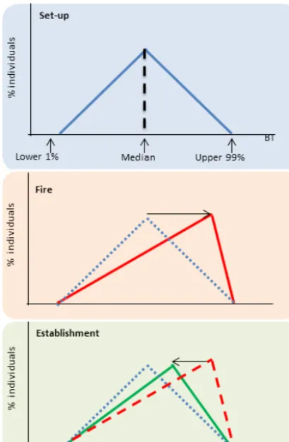
Figure 5. Illustration of the variable bark thickness scheme. The initial set-up is based on parameter values (Table 1) obtained from Fig. 4. Fire preferentially kills individual plants with thin bark, changing the distribution towards individuals with thicker bar. Es-tablishment shifts the distribution back towards the initial set-up.
ca. 50 % of leaf mass being recovered within a year and full recovery within ca. 5–7 yr (Viedma et al., 1997; Calvo et al., 2003; Casady, 2008; Casady et al., 2009; Gouveia et al., 2010; van Leeuwen et al., 2010; Gharun et al., 2013, see Fig. 7 and Table S3 in the Supplement).
However, species that resprout from aerial tissue (apical or epicormic resprouters in the terminology of Clarke et al., 2013) either need to have thick bark (see e.g. Midgley et al., 2011) or some other morphological adaptation to protect the meristem (e.g. see Lawes et al., 2011a, b). Investment in re-sprouting appears to be at the cost of seed production: in gen-eral, resprouting trees produce much less seed and therefore have a lower rate of post-disturbance establishment than non-resprouters (Midgley et al., 2010).
Aerial resprouting is found in both tropical and temper-ate trees, regardless of phenology (Kaufmann and Hartmann, 1991; Bellingham and Sparrow, 2000; Williams, 2000; Bond and Midgley, 2001; Del Tredici, 2001; Paula et al., 2009). It is very uncommon in gymnosperms (Del Tredici, 2001; Paula et al., 2009; Lunt et al., 2011) and does not seem to be promoted by fire in deciduous broadleaf trees in boreal
climates (Greene et al., 1999). We therefore introduced resprouting variants of four PFTs in LPX-Mv1: tropical broadleaf evergreen tree (TBE), tropical broadleaf deciduous tree (TBD), temperate broadleaf evergreen tree (tBE), and temperate broadleaf deciduous tree (tBD). Parameter values were assigned to be the same as for the non-resprouting vari-ant of each PFT, except for BT and establishment rate.
The species used in the bark thickness analysis were cat-egorised into aerial resprouters, other resprouters and non-resprouters (see Table S1 in the Supplement) based on field observations by the original data contributors, trait databases (e.g. http://www.landmanager.org.au; Kattge et al., 2011; Paula et al., 2009) or information in the literature (e.g. Harrison et al., 2014; Malanson and Westman, 1985; Pausas, 1997; Dagit, 2002; Tapias et al., 2004; Keeley, 2006).
Resprouting is facultative, and whether it is observed in a given species at a given site may depend on the fire regime and fire history of that site. Any species that was observed to resprout in one location was assumed to be capable of resprouting, even if it was classified as a non-resprouter in some studies. The range of BT for each resprouting (RS) PFT was calculated as in Sect. 3.5 (see Fig. 4 and Table 1). The range of BT was also re-assigned for their non-resprouting (NR) counterparts using species classified as having no re-sprouting ability.
The BT and post-fire mortality of RS PFTs is calculated in the same way as for NR PFTs. The allocation of fire-killed material in RS PFTs to fuel classes is also the same as for NR PFTs. However, after fire events, the RS PFTs are not killed, as described in Eq. (7), but allowed to resprout. The new average plant for RS PFTs is calculated as the average of trees not affected by fire and fire-affected trees RS trees.
4 Model configuration and test
Each change in parameterisation was implemented and eval-uated separately. For each change, the model was spun-up using detrended climate data from the period 1950– 2000 and the standard lightning climatology (following the protocol outlined in Prentice et al., 2011) until the car-bon pools were in equilibrium. The length of the spin-up varies but is always more than 5000 yr. After spin-spin-up, the model was run using a monthly lightning climatol-ogy from the Lightning Imaging Sensor–Optical Transient Detector high-resolution flash count (http://gcmd.nasa.gov/ records/GCMD_lohrmc.html), time-varying climate data de-rived from the CRU (Mitchell and Jones, 2005) and Na-tional Centers for Environmental Prediction (NCEP) reanal-ysis wind (NOAA Climate Diagnostics Center, Boulder, Col-orado; http://www.cdc.noaa.gov/) data sets as described in Prentice et al. (2011). We took the opportunity to correct an error in the NCEP wind inputs used by Kelley et al. (2013) but, given that this correction was made for all of LPX-Mv1 runs, this change has no impact on the differences caused by the new parameterisations.
We used the benchmarking system of Kelley et al. (2013) to evaluate the impacts of each change on the simulation of fire and vegetation processes. This benchmarking sys-tem quantifies differences between model outputs and obser-vations using remotely sensed and ground obserobser-vations of a suite of vegetation and fire variables and specifically de-signed metrics to provide a “performance score”. We make the comparison only for the continent of Australia, since this is a highly fire-prone region (van der Werf et al., 2008; Giglio et al., 2010; Bradstock et al., 2012) and was the worst sim-ulated in the original model (see Kelley et al., 2013). We used the benchmark observational data sets described in Kel-ley et al. (2013), with the exception of CO2concentrations,
runoff, GPP (gross primary production) and NPP. There are too few data points (<10) from Australia in the runoff, GPP and NPP data sets to make comparisons statistically mean-ingful. We did not use the CO2concentrations because this
requires global fluxes to be calculated.
We have expanded the Kelley et al. (2013) benchmark-ing system to include Australia-specific data sets for produc-tion and fire (Table 3). To benchmark producproduc-tion, we com-pared modelled 1 h fuel production to the Vegetation and Soil-carbon Transfer (VAST) fine-litter production data set for Australian grassland ecosystems (Barrett, 2001). Kelley et al. (2013) provide a burnt area benchmark based on the third version of the Global Fire Database (GFED3; Giglio et al., 2010). This has recently been updated (GFED4; Giglio et al., 2013). We re-gridded the data for the period (i.e. the period for which we have climate data to drive the LPX-Mv1 simulations) to 0.5◦resolution to serve as a benchmark for the model simulations, although we continue to use GFED3 for comparison with results from Kelley et al. (2013).We also use a burnt area product for southeastern Australia based on
ground observations of the extent of individual fires during the fire year (July–June) for the period from July 1970 to June 2009 on a 0.001◦grid (Bradstock et al., 2014). These
data were re-gridded to 0.5◦ resolution for annual average and interannual comparisons with simulated burnt area for July 1996–June 2005.
The difference between simulation and observation was assessed using the metrics described in Kelley et al. (2013). Annual average and interannual comparisons were con-ducted using the normalised mean error metric (NME). Sea-sonal length was benchmarked by calculating the concentra-tion of the variable in one part of the year for both model and observations, and comparing these concentrations with NME. Possible scores for NME run from 0 to∞, with 0 being a perfect match. Changes in NME are directly pro-portional to the change in model agreement to observations, therefore a percentage of improvement or degradation in model performance is obtained from the ratio of the origi-nal model to the new model score. NME takes a value of 1 when agreement is equal to that expected when the mean value of all observations is used as the model. Following Kelley et al. (2013), we describe model scores greater/less than 1 as better/worse than the “mean null model” and we also use random resampling of the observations to develop a second “randomly resampled” null model. Models are de-scribed as better/worse than randomly resampled if they were less/more than two standard deviations from the mean ran-domised score. The values for the randomly resampling null model for each variable are listed in Table 4.
For comparisons using NME, removing the influence of first the mean, and then the mean and variance, of both sim-ulated and observed values allowed us to assess the perfor-mance of the mapped range and spatial (for annual average and season length comparisons) or temporal (for interannual) patterns for each variable using NME.
We used the mean phase difference (MPD) metric to com-pare the timing of the season and the Manhattan metric (MM: Gavin et al., 2003; Cha, 2007) to compare vegetation type cover (Kelley et al., 2013). Both these metrics take the value 0 when the model agrees perfectly with the data. MPD has a maximum value of 1 when the modelled seasonal timing is completely out of phase with observations; whereas MM scores 2 when there is a perfect disagreement. Scores for the mean and random resampling null models for MM and MPD comparisons are given in Table 4.
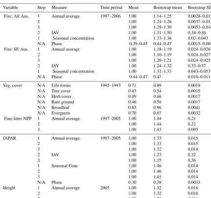
Table 3. Summary description of the benchmark data sets.
Data set Variable Type Period Comparison Reference
GFED4 Fractional burnt area Gridded 1996–2005 Annual average, seasonal phase and concentration, interannual variability
Giglio et al. (2013)
GFED3 Fractional burnt area Gridded 1996–2005 Annual average, seasonal phase and concentration, interannual variability
Giglio et al. (2010)
SE ground observations
Fractional burnt area Gridded 1996–2005 Annual average Bradstock et al. (2014)
VAST Above-ground
fine-litter production
Site 1996–2005 Annual average, interannual vari-ability
Barrett (2001)
ISLSCP II vegetation continuous fields
Vegetation fractional cover
Gridded Snapshot 1992/1993
Fractional cover of bare ground, herbaceous and tree; tree cover split into evergreen or deciduous, and broadleaf or needleleaf
DeFries and Hansen (2009)
SeaWiFS Fraction of absorbed photosynthetically ac-tive radiation (fAPAR)
Gridded 1998–2005 Annual average, seasonal phase and concentration, interannual variability
Gobron et al. (2006)
Canopy height Annual average height
Gridded 2005 Direct comparison Simard et al. (2011)
except resprouting is termed LPX-Mv1-nr and the run in-cluding resprouting is termed LPX-Mv1-rs.
4.1 Testing the formulation of resprouting
To assess the response of vegetation to the presence/absence of resprouting, we ran both LPX-Mv1-rs and LPX as de-scribed above for southeastern Australia woodland and for-est ecosystems with ≥20 % wood cover as determined by the International Satellite Land-Surface Climatology Project (ISLSCP) II vegetation continuous field (VCF) remotely sensed data set (Hall et al., 2006; DeFries and Hansen, 2009) (Fig. 8). Normal fire regimes were simulated until 1990, when a fire was forced burning 100 % of the grid cells, and killing (or causing to resprout, in the case of RS PFTs) 60 % of the plants. Fire was stopped for the rest of the simulation to assess recovery from this fire. As the proportion of indi-viduals killed was fixed, this experiment only tested the RS scheme and not factors affecting mortality. The LPX simula-tion therefore serves as a test for NR PFTs in LPX-Mv1 as well. The simulated total FPC in the post-fire years was com-pared against site-based remotely sensed observations of in-terannual post-fire greening following fire in fire-prone sites with Mediterranean or humid subtropical vegetation from several different regions of the world (Table S3), split into sites dominated by either RS and other fire adapted vegeta-tion (normally obligate seeders – OS) as defined in Sect. 3.6 based on the dominant species listed in each study (Table S3 in the Supplement). (The use of observations from other
regions of the world reflects the lack of observations of post-fire recovery in Australia.) We also used studies from bo-real areas with low fire frequency to examine the response in ecosystems where fire-response traits are uncommon (Table S3 in the Supplement). The comparison between simulated and observed regeneration was performed using a simple re-generation index (RI) that describes the percentage of recov-ery of lost normalised difference vegetation index (NDVI) at a given time,t, after an observed fire:
RIt=100·
QVIt−min QVIpostfire
QVIprefire , (35)
where QVIt is the ratio of the vegetation index (VI) of the burnt areas at timet after a fire compared to that of either an unburnt control site or, in studies where a control site was not used, the average VI of the years immediately preceding the fire; min(QVIpostfire)is the minimum QVI in the years
immediately following the fire; and QVIprefireis the average
QVI in the years immediately preceding the fire. NDVI was the most commonly used remotely sensed VI in the studies used for comparison. FPC has a linear relationship against NDVI (Purevdorj et al., 1998). However, this relationship differs between grass and woody plans (Xiao and Moody, 2005). As NDVI is normalised when used in Eq. (35), a di-rect conversion from FPC to NDVI is not necessary. Instead, we scaled for the different contributions from tree and grass, defining NDVIsim based on the statistical model described
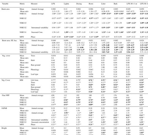
Table 4. Scores obtained using the mean of the data (data mean), and the mean and standard deviation (SD) of the scores obtained from randomly resampled null model experiments (Bootstrap mean, Bootstrap SD). Step 1 is a straight comparison; 2 is a comparison with the influence of the mean removed; and 3 is with mean and variance removed. The scores given for fire represent the range of scores over all fire data sets for that comparison. Scores for individual data sets can be found in Table S4 in the Supplement.
Variable Step Measure Time period Mean Bootstrap mean Bootstrap SD
Fire: All Aus. 1 Annual average 1997–2006 1.00 1.14–1.25 0.0028–0.015
2 1.00 1.24–1.26 0.0037–0.015
3 1.00 1.28–1.30 0.0053–0.016
2 IAV 1.00 1.31–1.50 0.34–0.36
1 Seasonal concentration 1.00 1.33–1.36 0.02–0.043
N/A Phase 0.39–0.45 0.44–0.47 0.0015–0.0046
Fire: SE Aus. 1 Annual average 1.00 1.18–1.19 0.024–0.026
2 1.00 1.10–1.19 0.024–0.027
3 1.00 1.20–1.21 0.024–0.025
2 IAV 1.00 1.24–1.32 0.33–0.37
1 Seasonal concentration 1.00 1.31–1.33 0.043–0.053
N/A Phase 0.44–0.47 0.47 0.010–0.011
Veg. cover N/A Life forms 1992–1993 0.71 0.89 0.0018
N/A Tree cover 0.43 0.54 0.0015
N/A Herb cover 0.49 0.66 0.0017
N/A Bare ground 0.46 0.56 0.0017
N/A Broadleaf 0.83 0.96 0.0041
N/A Evergreen 0.70 0.87 0.0032
Fine-litter NPP 1 Annual average 1997–2005 1.00 1.44 0.21
2 1.00 1.44 0.22
3 1.00 1.43 0.095
fAPAR 1 Annual average 1997–2005 1.00 1.33 0.015
2 1.00 1.33 0.015
3 1.00 1.32 0.014
2 IAV 1.00 1.23 0.32
3 1.00 1.35 0.36
1 Seasonal Conc 1.00 1.46 0.014
2 1.00 1.46 0.014
3 1.00 1.45 0.014
N/A Phase 0.30 0.38 0.0033
Height 1 Annual average 2005 1.00 1.32 0.016
2 1.00 1.32 0.016
3 1.00 1.31 0.016
Supplement, Eqs. S1–S4):
NDVIsim=FPCtree+0.32·FPCgrass, (36)
where FPCtreeis the fractional cover of trees and FPCgrassof
grasses.
A site or model simulation was considered to have re-covered when vegetation cover reached 90 % of the pre-fire cover (i.e. when RI=90 %). Recovery times for each site are listed in Table S3. Note that RI is a measure of the recovery of vegetation cover, not recovery in productivity or biomass. If a site or model simulation simulation failed to recover be-fore the end of the study, the recovery point was calculated by extending RI forward by fitting the post-fire data from the
site to RI=100·
1− 1
1+p·t
, (37)
Table 5. Scores obtained for the individual parameterisation experiments, and for the LPX-Mv1-nr and LPX-Mv1-rs experiments com-pared to the scores obtained for the LPX experiment. The metrics used are NME, MPD and the MM. S1 are step 1 comparisons, S2 are step 2, and S3 are step 3. The individual parameterisation experiments are Lightn: lightning re-parameterisation, Drying: fuel drying-time re-parameterisation, Roots: rooting depth re-parameterisation, Litter: litter decomposition re-parameterisation, and Bark: inclusion of adap-tive bark thickness. LPX-M-v1-nr incorporates all of these parameterisations and LPX-M-v1-rs incorporates resprouting into LPX-Mv1-nr. Numbers in bold are better than the original LPX model; numbers in italics are better that the mean null model; and * means better than the randomly resampled null model. The scores given for fire represent the range of scores over all fire data sets for that comparison. Scores for comparisons against individual data sets can be found in Table S5 in the Supplement.
Variable Metric Measure LPX Lightn Drying Roots Litter Bark LPX-M v1-nr LPX-M v1-rs
Burnt area Mean Annual Average 0.082 0.12 0.084 0.086 0.02 0.003 0.049 0.050
Mean ratio 1.13–1.21 1.64–1.77 1.15–1.24 1.18–1.27 0.28–0.29 0.039–0.043 0.67–0.72 0.69–0.74
NME S1 Annual Average 1.00*–1.01* 1.24*–1.29 1.00*–1.02* 1.00*–1.02* 0.90*–0.93* 0.88*–0.90* 0.88*–0.89* 0.85*–0.88*
NME S2 0.97*–0.97* 1.06*–1.09* 0.97*–0.98* 0.97*–0.97* 1.03*–1.04* 1.02*–1.02* 0.90*–0.94* 0.89*–0.93*
NME S3 1.20*–1.22* 1.32–1.32 1.21*–1.23* 1.20*–1.23* 1.22–1.23* 1.38–1.39 1.10*–1.12* 1.09*–1.09*
NME S2 Interannual variability 0.94–1.05* 1.05*–1.06 0.97*–1.08* 0.97*–1.17* 0.89–1.03* 1.00*–1.03* 0.66*–0.91 0.68*–0.90*
NME S1 Seasonal Conc. 1.39-1.43 1.30*–1.33 1.35*–1.43 1.36*–1.44 1.31*–1.44 1.31*–1.44* 1.31*–1.32* 1.31*–1.32*
MPD Phase 0.44*–0.50 0.38*–0.46* 0.44*–0.50 0.44*–0.49* 0.57–0.57 0.53–0.59 0.49*–0.52 0.49*–0.52
Burnt area: SE Aus. Mean Annual Average 0.048 0.099 0.053 0.051 0.012 0.002 0.024 0.024
Mean ratio 6.00–10.9 12.4–22.6 6.68–12.2 6.37–11.6 1.55–2.83 0.25–0.49 3.07–6.61 3.12–5.68
NME S1 Annual Average 4.03–7.19 7.97–14 4.35–7.67 4.23–7.59 1.59–2.40 0.81*–0.92* 2.29–4.27 2.33–3.67
NME S2 3.58–6.13 5.07–7.91 3.6–6.06 3.61–6.21 1.78–2.99 1.05*–1.08* 2.50–4.75 2.53–4.20
NME S3 1.41–2.07 1.23–1.35 1.35–1.37 1.38–1.40 1.22–1.25 1.18*–1.22 1.29–1.29 1.28–1.30
NME S2 Interannual variability 8.59–16.6 10.1–19.3 9.05–17.5 10.1–19.4 3.83–7.65 1.27–2.33 5.56–11.5 5.71–11.2
Veg. cover Mean Trees 0.034 0.011 0.022 0.034 0.059 0.075 0.042 0.049
Mean ratio 0.4 0.13 0.26 0.4 0.69 0.88 0.49 0.58
Mean Herb 0.44 0.34 0.45 0.44 0.55 0.57 0.55 0.55
Mean ratio 0.65 0.5 0.65 0.65 0.81 0.84 0.80 0.81
Mean Bare ground 0.52 0.65 0.53 0.52 0.39 0.35 0.41 0.4
Mean ratio 2.79 3.45 2.83 2.77 2.08 1.88 2.18 2.12
Mean Phenology 0.066 0.014 0.042 0.063 0.12 0.15 0.10 0.12
Mean ratio 0.13 0.026 0.081 0.12 0.23 0.28 0.20 0.22
Mean Leaf type 0.055 0.01 0.035 0.056 0.1 0.14 0.096 0.11
Mean ratio 0.094 0.018 0.059 0.096 0.18 0.24 0.17 0.18
Veg. Cover MM Life form 0.77* 0.96 0.79* 0.76 * 0.59 * 0.56 * 0.59 * 0.58*
Trees 0.16* 0.17* 0.17* 0.17* 0.17* 0.19* 0.17* 0.16*
Herb 0.66 0.77 0.67 0.65* 0.53* 0.52* 0.51* 0.51*
Bare ground 0.72 0.95 0.73 0.71 0.49 * 0.42 * 0.51 * 0.49*
Phenology 0.29* 0.33* 0.24* 0.29* 0.61* 0.81* 0.72 0.46
Leaf type 0.51* 1.01 0.62* 0.46* 0.34* 0.27* 0.15* 0.19*
Fine NPP Mean Annual average 628 112 192 180 177 176 181 202
Mean ratio 2.67 0.5 0.85 0.8 0.78 0.80 0.82 0.90
NME S1 2.62 0.96* 0.79* 0.78* 0.82* 1.13* 0.80* 0.73*
NME S2 1.47 0.83* 0.79* 0.78* 0.83* 1.22* 0.79* 0.74*
NME S3 0.97* 0.91* 1.01* 0.89* 1.01* 2.00 0.99* 0.87*
fAPAR Mean Annual average 0.19 0.12 0.19 0.18 0.24 0.26 0.22 0.22
Mean ratio 1.59 1.02 1.56 1.55 2.02 2.18 1.83 1.87
NME S1 Annual average 1.11* 0.98 * 1.11* 1.07 * 1.61 1.8 1.31 1.35
NME S2 0.69 * 0.97 * 0.72 * 0.68 * 0.7 * 0.69 * 0.61 * 0.61 *
NME S3 0.71 * 1.21* 0.76 * 0.71 * 0.57 * 0.51 * 0.57 * 0.54 *
NME S2 Interannual variability 1.01 1.11 1.01 0.97 2.44 2.86 1.83 1.85
NME S3 Seasonal concentration 1.34* 1.44 1.35* 1.36* 1.31* 1.31* 1.32* 1.33 *
MPD Phase 0.25 * 0.25 * 0.25 * 0.24 * 0.25 * 0.25 * 0.24 * 0.24*
Height Mean Annual Average 0.5 0.2 0.29 0.5 0.84 1.03 0.39 0.63
Mean ratio 0.056 0.022 0.033 0.057 0.096 0.12 0.045 0.072
NME S1 1.07* 1.1* 1.09* 1.07* 1.02* 1.01* 1.08* 1.05*
NME S2 0.94* 0.98* 0.97* 0.94* 0.91* 0.9* 0.96* 0.94*
NME S3 1.25* 1.39 1.31* 1.26* 1.11* 1.08* 1.18* 1.13*
5 Model performance
Evaluation of the model simulations focuses on changes in vegetation distribution (expressed through changes in the rel-ative abundance of PFTs) and changes in burnt area (both to-tal area burnt each year in each grid cell, i.e. fractional burnt
Figure 6. Comparison of the simulated abundance of grass, trees and resprouting trees along the climatic gradient in moisture, as measured by α (actual potential evapotranspiration). Remotely sensed observations (a) of tree and grass cover from DeFries and Hansen (2009) compared to distribution of grass and trees simulated (b) by LPX and (c) LPX-Mv1-rs. (d) Observations of the abundance of aerial resprouters (RS – red) and other species (NR – black) from Harrison et al. (2014) compared to (e) RS (red) and non-resprouting (NR) PFTs (black) simulated by LPX-M-v1-rs. Note that some of the species included in the observed NR category may exhibit post-fire recovery behaviours such as underground (clonal) regrowth.α
was calculated as described by Gallego-Sala et al. (2010) in (a) and (d), and simulated by the relevant model in (b), (c) and (e). Abun-dance in (d) and (e) is normalised to show the percentage of the total vegetative cover of each category. Solid lines denote the 0.1 running mean and shading denotes the density of sites based on quantiles for each 0.1 running interval ofα.
1990 1995 2000 2005 2010
0
20
40
60
80
100
year
reco
v
er
y inde
x (%) LPX − RS
LPX − NR Obs − RS Obs − OS Obs − NR LPX − RS LPX − NR Obs − RS Obs − OS Obs − NR
Figure 7. Comparison of the time taken for leaf area (as indexed by total foliage projective cover, FPC), to recover after fire in differ-ent ecosystems, as shown in the LPX-Mv1-rs simulations and from observations listed in Table S3. For comparison with the observa-tions, which were all made after a significant loss of above-ground biomass through fire, the LPX simulations show recovery after a loss of 60 % of the leaf area. Red denotes ecosystems dominated by above-ground RS species; blue denotes ecosystems dominated by other fire-adapted species, mostly OS; black denotes vegetation which does not display specific fire adaptations (NR). The solid lines show LPX simulations; dotted lines show the mean of the rel-evant observations; the shaded areas show interquartile ranges of the relevant observations. The plots show that LPX-M-v1 repro-duces the observed recovery rate in ecosystems dominated by re-sprouting species; recovery in ecosystems lacking rere-sprouting trees is slower than observed, which could either reflect issues with sim-ulated growth rates or the absence of other forms of fire adaptation.
simulations. We use benchmarking metrics to quantify the differences between the simulations (Table 5, Table S5 in the Supplement). Following (Kelley et al., 2013), we calculate the metrics in three steps in order to take account of biases: Step 1 is a straight comparison; 2 is a comparison with the influence of the mean removed; and 3 is with mean and vari-ance removed.
As the NME and MM metrics are the sum of the abso-lute spatial variation between the model and observations, the comparison of scores obtained by two different models shows the relative magnitude of their biases with respect to the observations, and the improvement can be expressed in percentage terms. Although we focus on vegetation distribu-tion and fire, we have also evaluated model performance in terms of other vegetation characteristics, including fAPAR, net primary production, and height (Table S5 in the Supple-ment), to ensure that changes in the model do not degrade the simulation of these characteristics.
5.1 LPX-Mv1-nr
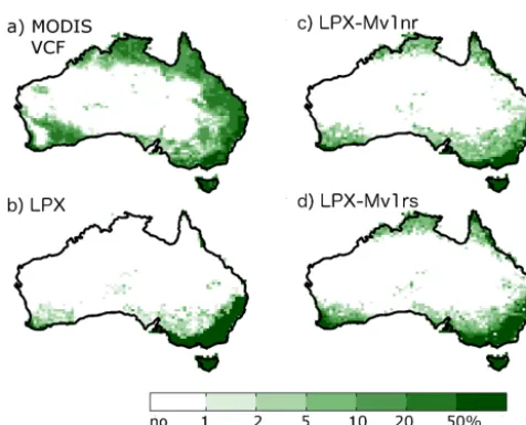
Figure 8. Comparison of percentage of tree cover from (a) obser-vations (DeFries and Hansen, 2009) and as simulated by LPX-M, LPX-Mv1-nr and LPX-Mv1-rs (b–d, respectively).
0.88–0.89 (better than the mean model) compared to scores for LPX of 1.00–1.01 (performance equal to or worse than the mean model). The change in NME (Table 5) is equiva-lent to a 13–14 % improvement in model performance. The improvement in annual burnt area can be attributed to an improved match to the observed spatial pattern of fire and a better description of spatial variance. The improved NME scores obtained after removing the influence of the mean and variance of both model outputs and observations (step 3 in Table 5) is due to the introduction of fire into climates with-out a pronounced dry season, such as swith-outheastern Australia (Fig. 9) which results from the lightning re-parameterisation (Fig. S1 in the Supplement). The improvement in spatial variability (step 2 in Table 5) is a result of a decrease in fire in the arid interior of the continent and an increase in fire in seasonally dry areas of northern Australia (Fig. 9). The decrease in fire in fuel-limited regions of the interior is a result of a decrease in fuel load from faster fuel composition, resulting from the re-parameterisation of de-composition, and a decrease in grassland production result-ing from the rootresult-ing depth re-parameterisation which leads to a decrease in the proportion of grass roots in the lower soil layer and increased water stress. Comparison of the sim-ulated fine-fuel production with VAST observations shows that the re-parameterisation of rooting depth improves simu-lation of fine-tissue production by 228 %. The improvement in the amount of fire in seasonally dry regions is a result of the re-parameterisation of fuel drying rates (Fig. S1 in the Supplement).
LPX-Mv1-nr produces an improved simulation of the in-terannual variability (IAV) of fire by 15–42 % from an NME of 0.94–1.05 to 0.66–0.91 (Table 5) – now better than the mean null model score of 1.00 (Table 4). This improvement
was due to the combination of the re-parameterisation of fuel drying time, which describes the impact of drier-than-normal conditions in certain years on fire incidence in northern and southeastern Australia, and a better description of litter de-composition in fine-fuel-dominated grassland, which allows for a more realistic description of fuel limitation in dry years where last year’s fuel has decomposed and no new fuel is being produced.
The simulation of the length of the fire season also im-proved by 6–8 %. The imim-proved NME score of 1.31–1.32 is better than the randomly resampled null model (1.332– 1.36±0.02–0.043), but not the mean model 1.00 (Table 4). Improvements come from the parameterisation of lightning, drying times and fuel decomposition. The new lightning pa-rameterisation leads to an increase in the length of the fire season, because fire starts occur over a longer period in coastal regions. The changes in drying time produce an ear-lier start to the fire season in all regions of Australia. The change to the decomposition parameterisation leads to a de-crease in fire in the arid interior of Australia towards the end of the dry season by reducing fuel loads.
Despite an improvement of 68–76 %, LPX-Mv1-nr still performs poorly for southeastern Australia when compared against ground observations. The score is better when satel-lite observations are used for comparison but NME scores are still worse than the randomly resampled null model (Ta-bles S4 and S5 in the Supplement). The model simulates too much fire in the Southern Tablelands (Fig. 9) but simulation of fire in more heavily wooded regions is more accurate, with burnt areas of ca. 1–5 %, in agreement with observations.
The improvement in vegetation distribution is largely due to simulating more realistic transitions between forest and grassland, chiefly through the parameterisation of adaptive bark thickness (which by itself yields a 37 % improvement in performance) but also through improved competition be-tween trees and grasses for water, which results from the re-parameterisation of rooting depth. The degradation of the MM score for tree cover only (0.17 or LPX-Mv1-nr com-pared to 0.16 for LPX) is because the new model simulates slightly too much tree cover in southeastern Australia. The boundaries between closed forests and savanna in this region are still too sharp (Fig. 8).
Figure 9. Annual average burnt area between 1997 and 2005 based on observations from (a) GFED3 (Giglio et al., 2010) and (b) GFED4 (Giglio et al., 2013), (c) southeastern Australia ground ob-servations (Bradstock et al., 2014), and as simulated by (d) LPX, (e) LPX-Mv1-nr, and (f) LPX-Mv1-rs.
high fAPAR forest near the coast and lower fAPAR grassland and desert in the interior. An MM comparison for phenology in areas where both LPX and LPX-Mv1-nr have woody cover shows little change in simulated phenology, with both scor-ing 0.29.
5.2 LPX-Mv1-rs
Including resprouting in LPX-Mv1 (LPX-Mv1-rs) produces a more accurate representation of the transition from for-est through woodland/savanna to grassland (Fig. 8) and im-proves the simulations of vegetation cover by 2 % compared to LPX-Mv1-nr and tree cover by 6 %. There is also a sig-nificant improvement in phenology compared to LPX-Mv1-nr, with NME scores changing from 0.72 in LPX-Mv1-nr to 0.46 in LPX-Mv1-rs (Table 5). The simulation of burnt area also improves: the NME for LPX-Mv1-rs is 0.85–0.88 com-pared to 0.88–0.89 for LPX-Mv1-nr, representing an overall improvement of 1–4 %. This improvement is equally due to the decrease in burnt area resulting from increased tree cover in southwestern Queensland (QL) and southeastern Australia (Fig. 10).
The simulated distribution of trees in climate space is im-proved in LPX-Mv1-rs compared to LPX. Trees are slightly more abundant at values ofα(the ratio of actual to equilib-rium evapotranspiration) between 0.2 and 0.4 in LPX-Mv1-rs than in LPX; while in humid climates, whereα >0.8, trees
Figure 10. The difference in (a) tree cover and (b) burnt area be-tween the non-resprouting MV1-nr) and resprouting (LPX-Mv1-rs) versions of LPX.
are less abundant than in LPX. The simulated abundance of trees in LPX-Mv1-rs is in reasonable agreement with obser-vations (Fig. 6)
The simulated distribution of RS dominance over NR PFTs is plausible. The observations indicate that aerial (api-cal and epicormic) resprouters are most abundant at inter-mediate moisture levels (αvalues between 0.4 and 0.6) but occur at higher moisture levels; the simulated abundance of RS is maximal atαvalues between 0.4 and 0.5 and, although it declines more rapidly at higher moisture levels than shown by the observations, resprouting still occurs in moist envi-ronments. RS has a competitive advantage over NR whenα is between 0.5 and 0.8 (Fig. S2 in the Supplement).
The simulated regeneration after fire in RS-dominated communities in southeastern Australia is fast: NDVIsim
6 Discussion
The introduction of new parameterisations in the LPX DGVM improves the simulation of vegetation composition and fire regimes across the fire-prone continent of Australia. The overall improvements in performance in LPX-Mv1-rs compared to LPX are 15–18 % for burnt area, 17–38 % for interannual variability of fire, and 33 % for vegetation com-position. These improvements result from the combination of all the new parameterisations. The introduction of indi-vidual parameterisations frequently led to a degradation of performance because LPX, in common with many other fire-enabled DGVMs, was tuned to produce a reasonably real-istic simulation of burnt area. Our approach here has been to develop realistic parameterisations based on analysis of large data sets; the model was not tuned against fire observa-tions. Post-fire aerial resprouting behaviour has not been in-cluded in DGVMs until now, although resprouting has been included in forest succession models (e.g. Loehle, 2000) and the BORFIRE (Boreal Fire Effects) stand-level fire-response model (Groot et al., 2003). Adaptive bark thickness has not been included in any vegetation model before, despite con-siderable within- and between-ecosystem variation in this trait and the fact that the average thickness within an ecosys-tem shifts with changes in fire regime. The incorporation of both processes is responsible for a significant part of the over-all model improvement in LPX-Mv1-rs vs. LPX; it produces more realistic vegetation transitions from forests to wood-land/savanna and, as shown by the regrowth comparisons, a more dynamically responsive DGVM.
The ability to resprout is a fundamental characteristic of many woody plants in fire-prone regions and means that these ecosystems recover biomass much more quickly af-ter fire than if regeneration occurs from seed. Thus, in ad-dition to improving the modern simulations, the incorpora-tion of resprouting in LPX-Mv1 should lead to a more ac-curate prediction of vegetation changes and carbon seques-tration in response to future climate-induced changes in fire regimes. The rapid post-fire regeneration in RS-dominated ecosystems is well reproduced using the modelling frame-work adopted here. However, simulated NR ecosystem re-covery is slower than observations (Fig. 7). This might, at least in part, be because the model does not yet include fire-recovery strategies found in other ecosystems. There are other post-fire recovery mechanisms including resprouting from basal or underground parts of trees and obligate seed-ing (Clarke et al., 2013). We focused on aerial resprout-ing because this has the fastest impact on ecosystem recov-ery (Crisp et al., 2011; Clarke et al., 2013) and thus the greatest potential to influence carbon stocks and vegetation patterns. However, basal/collar resprouting is important in shrubs (Harrison et al., 2014), and thus should be included in models that simulate shrub PFTs explicitly. The “obligate seeder” strategy (i.e. the release of seeds from canopy stores by fire or the triggering of germination of seeds stored in
the soil by smoke or fire-produced chemicals) also leads to a more rapid recovery than non-stimulated regeneration from seed. Obligate seeders are found in a wider range of ecosys-tems than resprouters, including boreal ecosysecosys-tems.
The ability to include a wider range of post-fire responses is currently limited by the availability of large data sets which could be used to develop appropriate parameterisations. Syn-thesis of the quantitative information available from the vast number of field studies on these traits would be useful for the modelling community. A similar argument could be made for information on rooting depth: although this is a trait that varies considerably within PFTs and depending on environ-mental conditions (Schenk and Jackson, 2002b, 2005), lack of species-level data has prevented us from implementing an adaptive deep root fraction within LPX-Mv1.
Despite the improvement in the simulation of fire in south-eastern Australia, LPX-Mv1-rs simulates ca. 5 times more fire than observed in some parts of Queensland, New South Wales and Victoria, where, although the natural vegetation is woodland/savanna, the proportion of the land used for agriculture (crops, pasture) is high, i.e.>80 % (Klein Gold-ewijk et al., 2011). The overall impact of agriculture is to reduce burnt area dramatically (Archibald et al., 2009; Bow-man et al., 2009), through increasing landscape fragmenta-tion (Archibald et al., 2012) and preventing fires from spread-ing. Incorporating land fragmentation into LPX-Mv1 could provide a more realistic simulation of fire in agricultural ar-eas, such as in southeastern Australia.