Use Hull White tree

USING HULL-WHITE INTEREST-RATE TREES

John Hull and Alan White

Rotman School of Management, University of Toronto 105 St. George Street, Toronto, Ontario, Canada M5S 3E6

Telephone Numbers John Hull: (416) 978-8615 Alan White: (416) 978-3689

USING HULL-WHITE INTEREST-RATE TREES ABSTRACT

The Hull-White tree-building procedure was first outlined in the Fall 1994 issue of Journal of Derivatives. It is becoming widely used by practitioners. This procedure is appropriate for models where there is some function x = f(r) of the short rate r that follows a mean-reverting arithmetic process. It can be used to implement the Ho-Lee model, the Hull-White model, and the Black-Karasinski model. Also, it is a tool that can be used for developing a wide range of new models.

In this article we provide more details on the way in which Hull-White trees can be used. We discuss the analytic results available when x = r and make the point that it is important to distinguish between the ∆ t-period rate on the tree and the instantaneous short rate that is used in some of these analytic results. We provide an example of the implementation of the model using market data. We show how the model can be implemented so that it provides an exact fit to the initial volatility environment while at the same time explaining why we do not recommend this approach. We also discuss how to deal with such issues as variable time steps, cash flows that occur between nodes, barrier options, and path

USING HULL-WHITE INTEREST-RATE TREES

In a recent Journal of Derivatives article, Hull and White [1994a], we described a procedure for constructing trinomial trees for one-factor yield curve models of the form:

( )

dx=θ − + σ (1)

where r is the short rate, x = f(r) is some function of r, a and are constants, and θ(t) is a function of time chosen so that the model provides an exact fit to the initial term structure of interest rates. The model can be written

( )

a t a

dx θ + σ

  

 ₋

=

This shows that, at any given time, x reverts toward θ(t)/a at rate a. Its variance rate per unit time is σ2.

When f(r)= r, the model reduces to the Hull-White [1990] model.

( )

[

]

dr= θ − + σ (1A)

The attraction of the Hull-White model is its analytic tractability. As shown in Hull and White [1990, 1994a] bonds and European options at some future time t can be valued analytically in terms of the initial term structure and the value of r at time t. When f(r) = log(r) and a and ### are allowed to be functions of time the model becomes Black and Karasinski [1991]. When f(r) = log(r) and a(t) = − σ'(t)/σ(t), and σ'(t) = ∂σ /∂t, the model becomes the Black, Derman, and Toy [1990] model. In Section III below we describe how to extend the basic tree-building procedure to accommodate time-varying mean reversion and volatility.

The construction of the Hull-White tree involves two stages. The first stage involves defining a new variable x* obtained from x by setting both θ(t) and the initial value of x

equal to zero. The process for x* is:

dz dt ax

dx*=− * + σ (2)

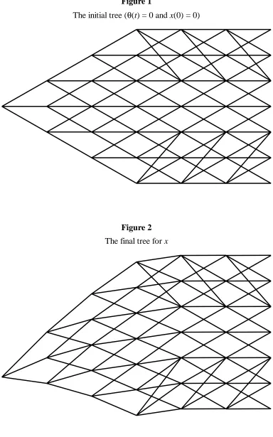
We construct a tree for x* that has the form shown in Figure 1. The central node at each time step has x* = 0. The vertical distance between the nodes on the tree is set equal to ∆x*= 3 where V V is the variance of the change in x in time ∆t, the length of each time step. The probabilities at each node are chosen to match the mean and standard deviation1

of the change in x* for the process in equation (2). Defining the expected change in x* as

Mx*, at node j ∆x* the up-, middle-, and down-branching probabilities are

1_{The expected value and variance of the change in x* over some time ∆t are}

[ ]

(

)

[ ]

(

)

2 6 1 3 2 2 6 1 2 2 2 2 2 2 jM M j p M j p jM M j p d m u − + = − = + + = (3A)

As indicated in Figure 1, we cope with mean reversion by allowing the branching to be nonstandard at the edge of the tree. At the top edge of the tree where the branching is non-standard the modified probabilities become

2 6 1 2 3 1 2 3 6 7 2 2 2 2 2 2 jM M j p jM M j p jM M j p d m u + + = − − − = + + = (3B)

and at the bottom edge of the tree where the branching is non-standard the modified probabilities become 2 3 6 7 2 3 1 2 6 1 2 2 2 2 2 2 jM M j p jM M j p jM M j p d m u − + = + − − = − + = (3C)

The second stage in the construction of the tree involves forward induction. We work forward from time zero to the end of the tree adjusting the location of the nodes at each time step in such a way that the initial term structure is matched. This produces a tree of the form shown in Figure 2. The size of the displacement is the same for all nodes at a particular time t, but is not usually the same for nodes at two different times. The effect of this second stage is to convert a tree for x* into a tree for x.

The full details of the tree building procedure are given in Hull and White [1994a]. In a later article, Hull and White [1994b], we describe extensions where two interest rates are modeled simultaneously and where the tree building technology is used to construct two-factor models of a single term structure.

The purpose of this article is to provide more details on the basic Hull-White tree building procedure. We discuss how to use analytic results when f(r)= r. We provide sample results based on a real yield curve that the reader can use to test his or her own

the time step can be changed, how cash flows that occur between time steps can be handled, and so on.

I. Analytic Results

Bond Prices:

When f(r)= r, the model in equation (1) is analytically very tractable. For example, as shown in Hull and White [1990, 1994a]

( ) ( )

P , = , − , (4)

where P(t, T) is the price at some time t of a zero coupon bond maturing at time T, r is the short-term rate of interest at time t, and A and B are functions only of t and T. The

function A is determined from the initial values of the discount bonds, P(0, T).

( ) ( )

_{( )}

[

( )

( )

(

)

( )

]

( )

(

)

, 2 2 2

− − − − = − − = σ (5)

F(0, t) is the instantaneous forward rate that applies to time t as observed at time zero. It can be computed from the initial price of a discount bond as F

( )

[

( )

]

The variable r in equation (4) is the instantaneous short rate while the interest rates on the Hull-White tree are ∆t-period rates. The two should not be assumed to be interchangeable. Let R be the ∆t period rate at time t, and r be the instantaneous rate at time t. Using equation (4):

(

)

e− ∆ = + ∆ − ,+∆

, so that

(

)

(

)

B t t t A t R r ∆ + ∆ + + ∆ = , , log (6)

To calculate points on the term structure given the ∆t period rate R at a node of the Hull-White tree it is first necessary to use equation (6) to get the instantaneous short rate, r. Equation (4) can then be used to determine rates for longer maturities. When this

procedure is followed, it can be shown that the prices of discount bonds that are computed are independent of the forward rate, F(0, t).2

Expected Future Rates:

Inspection of equations (1) and (2) shows that x(t) and x*(t) differ only by some function of time. Define this difference as

2_{Since the forward rate is computed from the first derivative of the yield curve it is very sensitive to the}

( ) ( )

( )

α (7)

This is the difference between the location of comparable nodes in the x and x* trees at time t. In particular it is the difference between the central or expected values of x and x* at time t, and since the expected value of x* is zero α(t) can be interpreted as the expected value of x(t). As has been pointed out by Kijima and Nagayama [1994] and Pelsser [1994], α(t) can be calculated analytically for the model where f(r)= r. Differentiating equation (7) it follows from equations (1) and (2) that

( ) ( ) ( )

t

α θ

∂

∂α _{= −}

or

( )

( )

( )

= t aq

dq e q r at t 0 0 exp θ α

Substituting the analytic expression for θ(t) given in Hull and White [1990, 1994a] this reduces to

( ) ( )

₍

₎

The use of the analytic expression for α to determine the location of the central nodes in the tree avoids the need to obtain them from forward induction.3 _{However, the resulting}

tree does not provide an exact fit to the initial term structure. This is because the tree is a discrete representation of the underlying continuous stochastic process. The advantage of the forward induction procedure is that the initial term structure is always matched exactly by the tree itself.

II. An Example

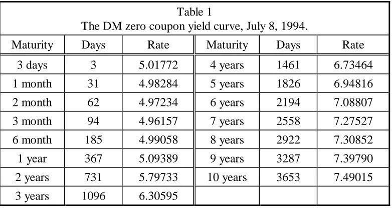
As an example of the implementation of the model we use the data in Table 1. This data, which is for the DM yield curve on July 8, 1994, was kindly provided to us by Antoon Pelsser of ABN Amro Bank.

Table 1

The DM zero coupon yield curve, July 8, 1994.

Maturity Days Rate Maturity Days Rate

3 days 3 5.01772 4 years 1461 6.73464

1 month 31 4.98284 5 years 1826 6.94816

2 month 62 4.97234 6 years 2194 7.08807

3 month 94 4.96157 7 years 2558 7.27527

6 month 185 4.99058 8 years 2922 7.30852

1 year 367 5.09389 9 years 3287 7.39790

2 years 731 5.79733 10 years 3653 7.49015

3 years 1096 6.30595

Data points for maturities between those indicated are generated using linear interpolation. The zero curve was used to price a 3-year4 (= 3 × _{365 day) put option on a zero coupon}

bond that will pay $100 in 9 years (= 9 × 365 days). Interest rates were assumed to follow the Hull-White (equation (1A)) model. The strike price was $63, and the parameters a and σ were chosen to be a = 0.1, and σ = 0.01. These two parameters determine the volatility of the discount bond for option pricing purposes. The values that were chosen were roughly representative of the values that are observed in the market. The tree was constructed out to the end of the life of the option. The zero-coupon bond prices at the final nodes were calculated analytically as described in the previous section.

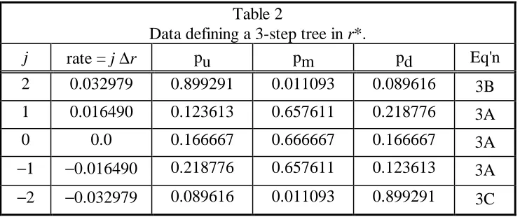
To illustrate the process consider the construction of a 3-step tree. First, we must determine the time and rate step sizes, and where non-standard branching (if any) takes place. The size of the time step is ∆t = 3 × 365 days / 3 / 365 days/year = 1.0 years. As shown in Hull and White [1994a] the expected change in r* and the variance of the change in r* in time ∆t are given by

[ ]

(

)

[ ]

(

)

E * = *= −a∆t − 1 *; Var * = =σ21− −2a∆t /2

For the given parameter values M = −0.095162582 and V = 0.009520222. Since the step size ∆r= 3 , ∆V r = 0.016489508. Finally, as shown in Hull and White [1994a] non-standard branching takes place at nodes ±j* where j* is the smallest integer greater than −0.184/M. In this case j* is 2. The data defining the initial tree is shown in Table 2.

4_{The fundamental unit of time in this example is one day. For convenience we define 1 year as 365 days,}

Table 2

Data defining a 3-step tree in r*.

j rate = j ∆r _{pu pm pd} Eq'n

2 0.032979 0.899291 0.011093 0.089616 _3B

1 0.016490 0.123613 0.657611 0.218776 3A

0 0.0 0.166667 0.666667 0.166667 _3A

−1 −0.016490 0.218776 0.657611 0.123613 _3A

−2 −0.032979 0.089616 0.011093 0.899291 _3C

The rates at each node in the tree at each time step are now shifted up by some amount, α, chosen so that the revised tree correctly prices discount bonds. Since there are nodes at the 1-, 2-, and 3-year points we need the discount bond prices corresponding to these dates as well as the 4-year price, one time-step beyond the option maturity. When the option price is calculated, the 9-year bond price will be required as well. This data,

interpolated from the data in Table 1 is shown in Table 3. Table 3 also shows the value of α required to fit the bond prices at each time step. An efficient procedure for implying the value of α is given in Hull and White [1994a]. For reference purposes the instantaneous forward rate and the instantaneous values of α (based on equation (8)) are also shown.

Table 3

The amount, α, by which the interest rates at each time step must be raised in order to replicate the bond prices computed from the zero coupon discount rates.

The instantaneous forward rate and the instantaneous value of α are also shown. Time Step

i

t = i ∆t

Years

Zero Rate (%)

Discount Bond Price

α (%)

Forward Rate (%)

α(t) - Eq'n (8) (%) 0 0.0 5.017720 1.000000 5.09275 5.017720 5.017720 1 1.0 5.092755 0.950348 6.50257 5.299942 5.304470 2 2.0 5.795397 0.890557 7.33932 7.206143 7.222572 3 3.0 6.304557 0.827673 8.05381 7.830417 7.864004

4 4.0 6.733466 0.763885

9.0 7.397410 0.513879

Table 4

The 4 time steps in the interest rate tree. The probability of transiting from node (i, j) to nodes (i+1, j+1), (i+1, j), and (i+1, j−_{1) are normally pu(}j), pm(j_{), and pd(}j) respectively. When j = ±2 the alternative branching schemes are used.

Transition Probabilities Node Rates, R, (%)

j _{pu pm pd} i = 0 i = 1 i = 2 i = 3

2 0.8993 0.0111 0.0896 10.6372 11.3517

1 0.1236 0.6576 0.2188 8.1515 8.9883 9.7028

0 0.1667 0.6667 0.1667 5.0928 6.5026 7.3393 8.0538

−1 0.2188 0.6576 0.1236 4.8536 5.6904 6.4049

−2 0.0896 0.0111 0.8993 4.0414 4.7559

Table 5

Computing the price of a bond that pays $1 at time 2 ∆t (2 years). Each value is calculated as

vi,j = (pu vi+1,j+1 + pm vi+1,j + pd vi+1,j−1) exp(-Ri,j ∆t). Transition Probabilities Bond Price

j _{pu pm pd} i = 0 i = 1 i = 2

2 0.8993 0.0111 0.0896 1.0

1 0.1236 0.6576 0.2188 0.9217 1.0

0 0.1667 0.6667 0.1667 0.8906 0.9370 1.0

−1 0.2188 0.6576 0.1236 0.9526 1.0

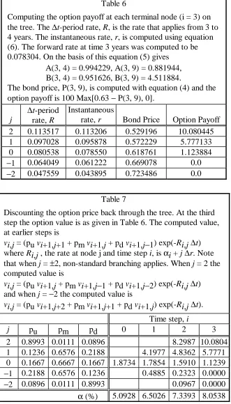
Table 6

Computing the option payoff at each terminal node (i = 3) on the tree. The ∆t-period rate, R, is the rate that applies from 3 to 4 years. The instantaneous rate, r, is computed using equation (6). The forward rate at time 3 years was computed to be 0.078304. On the basis of this equation (5) gives

A(3, 4) = 0.994229, A(3, 9) = 0.881944, B(3, 4) = 0.951626, B(3, 9) = 4.511884.

The bond price, P(3, 9), is computed with equation (4) and the option payoff is 100 Max[0.63 − P(3, 9), 0].

j

∆t-period rate, R

Instantaneous

rate, r Bond Price Option Payoff

2 0.113517 0.113206 0.529196 10.080445

1 0.097028 0.095878 0.572229 5.777133

0 0.080538 0.078550 0.618761 1.123884

−1 0.064049 0.061222 0.669078 0.0

−2 0.047559 0.043895 0.723486 0.0

Table 7

Discounting the option price back through the tree. At the third step the option value is as given in Table 6. The computed value, at earlier steps is

vi,j = (pu vi+1,j+1 + pm vi+1,j + pd vi+1,j−1) exp(-Ri,j ∆t)

where _Ri,j , the rate at node j and time step i, is α_i + j ∆r. Note that when j = ±2, non-standard branching applies. When j = 2 the computed value is

vi,j = (pu vi+1,j + pm vi+1,j−1 + pd vi+1,j−2) exp(-Ri,j ∆t)

and when j = −2 the computed value is

vi,j = (pu vi+1,j+2 + pm vi+1,j+1 + pd vi+1,j) exp(-Ri,j ∆t).

Time step, i

j _{pu pm pd} 0 1 2 3

2 0.8993 0.0111 0.0896 8.2987 10.0804

1 0.1236 0.6576 0.2188 4.1977 4.8362 5.7771 0 0.1667 0.6667 0.1667 1.8734 1.7854 1.5910 1.1239 −1 0.2188 0.6576 0.1236 0.4885 0.2323 0.0000

−2 0.0896 0.0111 0.8993 0.0967 0.0000

α (%) 5.0928 6.5026 7.3393 8.0538

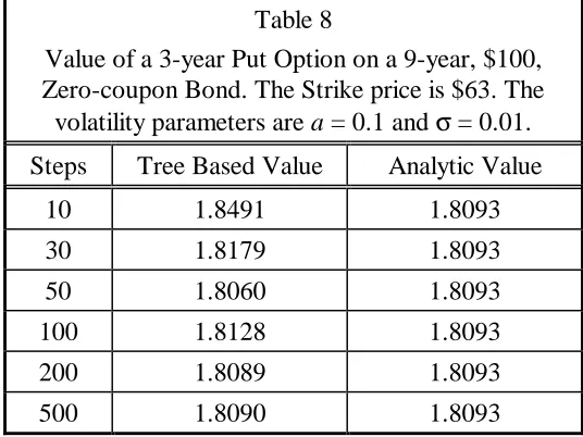
in the construction and use of the tree are liable to have a big effect on the option values obtained. For example, when 100 time steps are used, the value of the option is reduced by about $0.25 if the ∆t-period rate is assumed to be the instantaneous rate.

Table 8

Value of a 3-year Put Option on a 9-year, $100, Zero-coupon Bond. The Strike price is $63. The volatility parameters are a = 0.1 and σ = 0.01. Steps Tree Based Value Analytic Value

10 1.8491 1.8093

30 1.8179 1.8093

50 1.8060 1.8093

100 1.8128 1.8093

200 1.8089 1.8093

500 1.8090 1.8093

III. Making Volatility Parameters Time Dependent

When a and σ are functions of time the model in equation (1) becomes

( ) ( )

[

]

( )

dx= θ − + σ (9)

The three functions of time in this diffusion equation each play a separate role. The function θ(t) is chosen so that the prices of all discount bonds are matched at the initial time. The other two functions provide two extra degrees of freedom that allow us to match the initial volatility of all zero coupon rates and the volatility of the short rate at all future times. The tree can then be tuned to price not only the zero-coupon bonds, but also a set of interest-rate derivatives at their current market prices. The initial volatility of all rates depends on σ(0) and a(t). The volatility of the short rate at future times is

determined by σ(t). Unless σ(t) and a(t) are constants the volatility term structure is non-stationary.

Our tree building procedure can be extended to accommodate the model in equation (9). Analogously to the constant a and σ case we first build a tree for x* where

( )

( )

dx*=− * + σ

We first choose the times at which nodes will be placed, t_0, t_1, t_2, …, t_{n, where} t_{0 = 0 and} ti = i ∆t for i = 0, …, n. The vertical (x* dimension) spacing between adjacent nodes at time _{ti+1 is then set equal to 3Vi} where

( )

(

)

_{( )}

i t t a i

i t e a t

V =σ 2 ₁− −2 i ∆ _/2

Suppose that the value of x* at the jth node at time _ti is x*_{i, j}. The mean and standard deviation of x* at time _{ti+1 conditional on} x* = x*_{i, j} at time _ti are approximately x*_{i, j} +

( )

(

)

= −at ∆t i

i

e M

We match these by branching from x*_{i, j} to one of x*_{i+1, k−1,} x*_{i+1, k}, and x*_{i+1, k+1} where k is chosen so that x*_{i+1, k} is as close as possible to x*_{i, j} + _Mix*_{i, j} ∆t. We then calculate the displacements, α(t), necessary for the tree to match the initial term structure. The a(t) and σ(t) can be set in advance of the numerical procedure. Alternatively, it is not difficult to devise a numerical procedure that chooses a(t) and σ(t) so that the initial prices of caps or swap options (or both) are matched. When used for x = log(r) this type of tree building procedure has the advantage over Black and Karasinski [1991] that the length of the time step is under the control of the user.5

It seems appealing to take advantage of all the degrees of freedom in a model to exactly fit initial market data. However, the resulting non-stationarity in the volatility term structure may have many untoward and unexpected effects. To illustrate this we use the x = r

model:

( ) ( )

[

]

( )

dr= θ − + σ

and show the effect of matching cap prices.

Caps are usually priced using Black's model, under which the price at time zero of a caplet expiring at T on a rate that applies from T to T + τ is

( )

[

₍

_{) ( )}

_{( )}

]

2 1

,T N d XN d

T F Pe

C =τ −RT+τ + τ −

where P is the notional principal, R is the zero coupon rate with a maturity T + τ, F(T, T + τ) is the forward rate for the period T to T + τ and X is the cap rate.

(

)

(

)

( )

( )

( )

where v(T) is the volatility for the caplet expiring at T.

The data set that we will use for calibration consists of the market prices of at-the-money caps that are reset monthly (τ = 1 month). The particular v(T) function we assume for illustration purposes is shown in Figure 3.6 _{This has a similar shape to the v(T) function}

commonly observed in the market. We assume the term structure is flat at 7% continuously compounded.

In order to match the Black volatilities we first used them in conjunction with Black's model to calculate caplet prices. We then matched the caplet prices in two ways:

5_{We will explain in the next section how the length of the time step can be changed by the user in the}

Hull-White tree building procedure.

6_{This volatility curve is} ( )

[

(

)

]

0 1

1 bT c e v T

v = + + − −dT _{for T}≤ _{5, b =} −_{0.1, c = 0.5, d = 0.8, and v(0) = 0.2.}

1. We fixed the short rate standard deviation, σ, and allowed the reversion rate, a, to be a function of time; and

2. We fixed a and allowed σ to be a function of time.

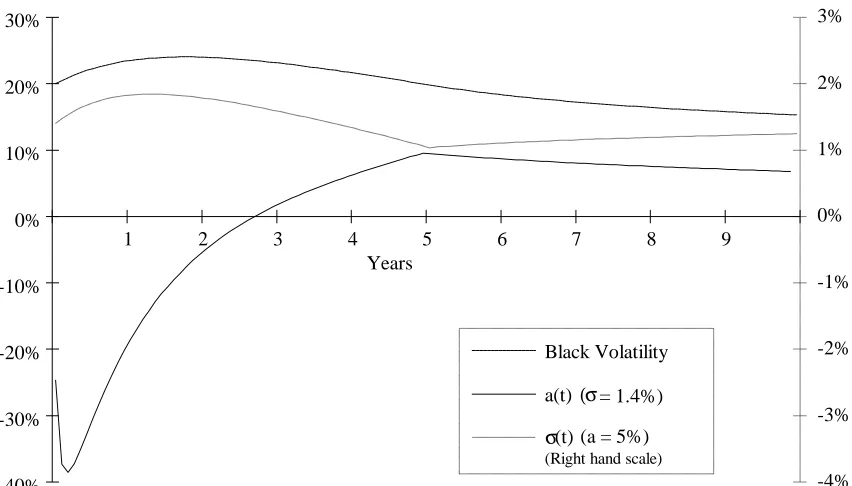
Figure 4 shows the value of a(t) required to fit the market data when σ is fixed7 _{at 1.4%}

and the value of σ(t) required to fit the market data when a is fixed at 5%. It can be seen that the implied a(t) and σ(t) exhibit severe non-stationarity. Although by construction this non-stationarity leads to caplets being priced correctly, it is liable to lead to unacceptable results when used to price other instruments.

Any instrument whose price depends on the future volatility structure, rather than today's volatility structure, is liable to be mispriced by a model with time dependent volatility parameters. One example of such a security is an American-style call option where the decision to exercise at some future date depends on the volatility structure at that date. Another example is a caption, an option to buy a cap, where the decision to exercise the option at it expiry depends on the value of the cap at that time.

This example illustrates the types of problems that can arise when a model is implemented in such a way that the volatility structure is not stationary. It is a problem that afflicts all Markov interest-rate models including the Black, Derman and Toy, and Black and Karasinski models. By fitting a one-factor Markov interest-rate model to today's option prices, we make it exactly reflect the initial volatility structure. However, we are also unwittingly making a statement about how the volatility term structure will evolve in the future. Using all the degrees of freedom in the model to fit the volatility exactly constitutes an over parameterization of the model. It is our opinion that there should be no more than one time varying parameter used in Markov models of the term structure evolution and that this should be used to fit the initial term structure.

IV. Other Issues

There are a number of other practical issues to consider when implementing Hull-White trees for valuing interest rate derivatives. In this section we review a number of these and indicate how they can be handled.

In our description of the tree-building procedure in Hull and White [1994a] it was assumed that the length of the time step is constant. In practice, it is sometimes desirable to change the length of the time step.8 _{Changing the length of the time step is}

straightforward. When drawing the tree for x*, we first choose the times at which nodes will be placed, t_0, t_1, t_2, …, t_{n, where} t_{0 = 0. Defining} ∆_ti = _ti+1 − _ti for i = 0, …, n − 1,

7_{The choice of the fixed value for} σ _{in this example, and the following choice of the fixed value for a are}

arbitrary. However, the implied values of a(t) and σ(t) are representative of the type of non-stationarity that results from the given volatility structure. The best fixed value of σ (or a) to use might be the one that minimizes the variance of the implied a(t) (or σ(t)).

8_{Consider for example the situation where the lognormal model is used to value a European 6-month}

the vertical (x* dimension) spacing between adjacent nodes at time _{ti+1 is then set equal} to 3_Vi where

(

)

V a ti

i 1 /2

2

2 − − ∆

=σ

From this point, the construction is similar to the procedure followed when the volatility parameters are a function of time. Suppose that the value of x* at the jth node at time _ti is

x*_{i, j}. The mean and standard deviation of x* at time _{ti+1 conditional on} x* = x*_{i, j} at time

ti are approximately x*_{i, j} + _Mix*_{i, j} and V_i , where

(

)

= −a∆ti

i e

M

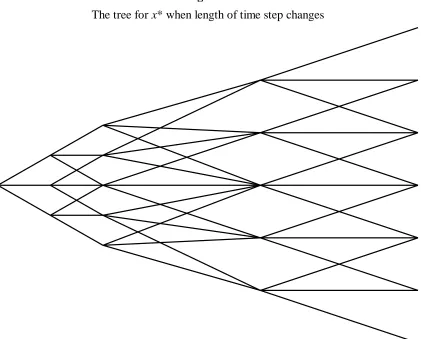
We match these by branching from x*_{i, j} to one of x*_{i+1, k−1,} x*_{i+1, k}, and x*_{i+1, k+1} where k is chosen so that x*_{i+1, k} is as close as possible to x*_{i, j} + _Mix*_{i, j} ∆_ti. Note that whenever the size of the time step changes, ∆_ti ≠ ∆_{ti+1, the vertical (}x* dimension) spacing between nodes increases by ∆t_i+1/∆t_i . This means that the branching is nonstandard at points when the length of the time step changes. Figure 5 illustrates the tree that is constructed when the time step increase by a factor of three after two time steps.

The tree for x is constructed from the tree for x* to match the initial zero coupon yield curve as described in Hull and White [1994a]. Note that, when the length of the time step changes from ∆_ti to ∆_{ti+1, the interest rates considered at the nodes automatically change} from the ∆_ti period rates to the ∆_{ti+1 rates.}

Another issue in the construction of the tree concerns cash flows that occur between nodal dates. Suppose a cash flow occurs at time τ when the immediately preceding nodal date is

ti and the immediately following nodal date is _{ti+1. One approach is to discount the cash} flow from time τ to the nodes at time _ti using estimates of the τ − _ti rates prevailing at the nodes at time _ti.9 Another approach is to assume that a proportion (τ − _ti)/(ti

+1 − ti) of the cash flow occurs at time _{ti+1 while the remainder occurs at time ti}.10 _{A final approach}

is to avoid the problem altogether by changing the length of the time step so that every payment date is also a nodal date.

Barrier options present a further problem in the use of the tree because convergence tends to be slow when nodes do not lie exactly on barriers. In the case of an interest rate option the barrier is typically expressed in terms of a bond price or a particular rate. When x = r, analytic results can be used to express the barrier as a function of the ∆t-period rate. Nonstandard branching can then be used to ensure that nodes always lie on the barrier. Ritchken (JOD Winter 1995) describes such an approach, and shows that a substantial improvement in performance is possible with it. An alternative approach that has more general applicability is to extend the idea suggested by Derman et al [1995] to interest rate

9_{In the case of the Hull-White, x = r model these rates can be calculated analytically.}

10_{This approach has the effect of apportioning the cash flow to nodal dates while ensuring that the}

trees. This approach involves using a procedure to correct values of the derivative calculated at nodes close to a barrier.

A final problem in the use of interest rate trees is path dependence. This can sometimes be handled in the way described by Hull and White [1993]. The requirements for the Hull-White method to work are:

1. The value of the derivative at each node must depend on just one function of the path for the short rate r (e.g., the maximum, minimum, or average value);

2. In order to update the path function as we move forward through the tree we need to know only the previous value of the function and the new value of r.

Hull and White show how their approach can be used for index amortizing swaps and mortgage-backed securities. The relevant path function in each case is the remaining principal.

V. Summary

REFERENCES

Black, F., Derman, E., and W. Toy, "A one-factor model of interest rates and its application to Treasury bond options,'' Financial Analysts Journal, (January-February, 1990), 33−39.

Black, F. and P. Karasinski, "Bond and option pricing when short rates are lognormal,''

Financial Analysts Journal, (July--August, 1991), 52−59.

Ho, T.S.Y. and S.-B. Lee, "Term structure movements and the pricing interest rate contingent claims,'' Journal of Finance, 41 (December 1986), 1011−29.

Hull, J. and A. White, "Pricing interest rate derivative securities,'' Review of Financial Studies, 3, 4 (1990), 573−92.

Hull, J. and A. White, "Efficient procedures for valuing European and American path-dependent derivatives,'' Journal of Derivatives, 1, 1 (Fall 1993) 21−31

Hull, J. and A. White, "Numerical procedures for implementing term structure models I: Single-Factor Models,'' Journal of Derivatives, 2, 1 (Fall 1994a) 7−16.

Hull, J. and A. White, "Numerical procedures for implementing term structure models II: Two-Factor Models,'' Journal of Derivatives, 2, 1 (Winter 1994b) 37−48.

Kijima, M. and I. Nagayama, "Efficient numerical procedures for the Hull-White extended Vasicek model,'' The Journal of Financial Engineering, 3, 4 (September/December 1994) 275−292.

Pelsser, A., "An efficient algorithm for calculating prices in the Hull-White model,'' ABN-Amro Bank, Derivative Product Research and Development working paper, 1994.

Ritchken, P, "On pricing barrier options,'' Journal of Derivatives, 3, 2 (Winter 1995) 19−

Figure 1

The initial tree (θ(t) = 0 and x(0) = 0)

Figure 2

Figure 3

Black's volatility for at-the-money caplets that are reset monthly

10 12 14 16 18 20 22 24 26

12 24 36 48 60 72 84 96 108 Months

Figure 4

Value of a(t) when σ = 1.4% (left-hand scale), and the value of σ(t) when a = 5% (right-hand scale) required to replicate the caplet prices computed from the Black volatilities in Figure 3. The Black volatilities from Figure 3 are included for reference purposes.

-40% -30% -20% -10% 0% 10% 20% 30%

1 2 3 4 5 6 7 8 9

-4% -3% -2% -1% 0% 1% 2% 3%

Black Volatility a(t)

σ(t)

(Right hand scale)

Figure 5