www.ann-geophys.net/26/107/2008/ © European Geosciences Union 2008
Annales
Geophysicae
The ionospheric responses to the 11 August 1999 solar eclipse:
observations and modeling
H. Le1,2, L. Liu1, X. Yue1,2, and W. Wan1
1Institute of Geology and Geophysics, Chinese Academy of Sciences, Beijing 100029, China 2Graduate School of the Chinese Academy of Sciences, Beijing 100049, China
Received: 27 August 2007 – Revised: 2 December 2007 – Accepted: 12 December 2007 – Published: 4 February 2008
Abstract. A total eclipse occurred on 11 August 1999 with
its path of totality passing over central Europe in the lat-itude range 40◦–50◦N. The ionospheric responses to this eclipse were measured by a wide ionosonde network. On the basis of the measurements of foE, foF1, and foF2 at six-teen ionosonde stations in Europe, we statistically analyze the variations of these parameters with a function of eclipse magnitude. To model the eclipse effects more accurately, a revised eclipse factor,FR, is constructed to describe the vari-ations of solar radiation during the solar eclipse. Then we simulate the effect of this eclipse on the ionosphere with a mid- and low-latitude ionosphere theoretical model by using the revised eclipse factor during this eclipse. Simulations are highly consistent with the observations for the response in the E-region and F1-region. Both of them show that the max-imum response of the mid-latitude ionosphere to the eclipse is found in the F1-region. Except the obvious ionospheric response at low altitudes below 500 km, calculations show that there is also a small response at high altitudes up to about 2000 km. In addition, calculations show that when the eclipse takes place in the Northern Hemisphere, a small ionospheric disturbance also appeared in the conjugate hemi-sphere.
Keywords. Ionosphere (Mid-latitude ionosphere; Modeling
and forecasting)
1 Introduction
Solar eclipses provide unique opportunities to study the be-havior of the ionosphere. During a solar eclipse, the Moon’s shadow decreases the ionizing radiation from the Sun, caus-ing changes in electron concentration and temperature, and neutral compositions and temperature. During the past
Correspondence to: L. Liu
decades, the responses of the ionosphere to solar eclipses have been studied extensively with various methods, such as the Faraday rotation measurement, ionosonde network, inco-herent scatter radar (ISR), Global Positioning System (GPS), and satellite measurements (e.g. Evans, 1965a, b; Klobuchar and Whitney, 1965; Rishbeth, 1968; Hunter et al., 1974; Oliver and Bowhill, 1974; Cohen, 1984; Salah et al., 1986; Cheng et al., 1992; Tsai and Liu, 1999; Huang et al., 1999; Afraimovich et al., 1998, 2002; Farges et al., 2001, 2003; Tom´as et al., 2007; Adeniyi et al., 2007). These studies have shown that there is almost a consistent behavior in the low altitudes where electron density drops by a large percentage during a solar eclipse, whereas the F2-region behavior may be quite complicated during different eclipse events, show-ing either an increase or decrease in electron density. In addition, responses of the low-latitude and equatorial sphere may be quite different from those in the middle iono-sphere. Huang et al. (1999) used a low-latitude ionospheric tomography network (LITN) to observe the ionospheric re-sponse to the solar eclipse of 24 October 1995 and found an enhancement, a depression, followed by an enhancement and depression in Total Electron Content (TEC). During the same eclipse event, there might be different ionospheric re-sponses in different locations because of the differences in background parameters.
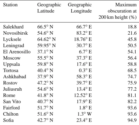
Table 1. Locations of the ionosonde stations used during the eclipse
measurements and their maximum solar obscuration at 200 km height.
Station Geographic Geographic Maximum Latitude Longitude obscuration at 200 km height (%)
Salekhard 66.5◦N 66.7◦E 18.8 Novosibirsk 54.6◦N 83.2◦E 21.6 Lycksele 64.62◦N 18.76◦E 45.8 Leningrad 59.95◦N 30.7◦E 50.5 El Arenosillo 37.1◦N 6.7◦E 54.1
Moscow 55.5◦N 37.3◦E 56.4
Uppsala 59.8◦N 17.6◦E 58.8
Tortosa 40.4◦N 0.3◦E 68.5
Ashkhabad 37.9◦N 58.3◦E 74.7
Rostov 47.2◦N 39.7◦E 75.9
Juliusruh 54.6◦N 13.4◦E 77.2
Rome 41.8◦N 12.52◦E 81.1
San Vito 40.7◦N 17.9◦E 82.2 Fairford 51.7◦N 1.8◦E 93.6
Chilton 51.6◦N 1.3◦W 93.6
Sofia 42.7◦N 23.4◦E 94.9
to the total solar eclipse in terms of a mid- and low-latitude ionosphere theoretical model. In the past, there have been some studies on the ionospheric response to solar eclipses on the basis of numerical simulations (e.g. Stubbe, 1970; Roble et al., 1986; M¨uller-Wodarg et al., 1998; Boitman et al., 1999; Liu et al., 1999; Korenkov et al., 2003a, 2003b). However, they only considered the occultation of the pho-tosphere being shielded by the Moon for variations in solar radiation during a solar eclipse. According to their method, the solar radiation should be zero when the photosphere is totally obscured, which would introduce some errors, espe-cially in the low altitudes, because even at totality there are still some radiations from the unmasked part of solar corona (Rishbeth, 1968; Davis et al., 2000; Curto et al., 2006). In this paper, according to the astronomical model of Curto et al. (2006), we construct a revised eclipse factor to describe the variation of solar radiation during a solar eclipse. Un-like earlier studies mentioned above, in addition to the re-sponse of the ionosphere in the Northern Hemisphere during the eclipse, we also find the ionospheric disturbance in the conjugate hemisphere.
2 Data source
The total eclipse of 11 August 1999 occurred with its path of totality passing over central Europe in the geographic lat-itude range 40◦N–50◦N. The eclipse occurred during a rel-atively long geomagnetic quiet period. The eclipse therefore provides a unique opportunity to study the mid-latitude iono-spheric response to the variation of solar EUV radiation. The
ionospheric responses to this eclipse were monitored by a wide ionosonde network. To examine the variations of the eclipse effects with the eclipse magnitude, which is defined as the fraction of the Sun’s diameter occulted by the Moon, we performed a statistical analysis of the critical frequency of the ionospheric E and F1 layer, foE and foF1, from 16 ionosonde stations. These stations are listed in Table 1, in the order of maximum obscuration. The maximum obscuration at 200 km altitude over each station ranges from around 20% to 95% as shown in Table 1. A mean of thirty days is used as a reference on the control day for comparing the ionospheric behavior of the E and F1 layer during the eclipse with the normal behavior. The ionosonde data often only have a time resolution of one hour or half an hour. So we calculate the ob-scuration at the time near totality when foE or foF1 is avail-able. Following a similar approach as Davis et al. (2000) and Curto et al. (2006), we calculated the relative changes in the peak electron density of the E layer and F1 layer, NmEE/NmECand NmF1E/NmF1C, as a function of the frac-tion of the Sun’s photosphere area unmasked by the Moon, SPE/SPCas seen at the height of 200 km, where NmEE and NmF1E are the peak electron densities of the E layer and F1 layer on the eclipse day, NmECand NmF1Care the peak electron densities of the E layer and F1 layer on the con-trol day, SPEis the Sun’s photosphere area unmasked by the Moon during the eclipse, SPCis the Sun’s photosphere area before and after the eclipse. The values of SPE/SPC can be obtained by astronomical calculation. According to the algo-rithm of Curto et al. (2006), the unmasked fraction of the to-tal solar ionizing radiation drops to a minimum of about 22% of the value before eclipse at totality (SPE/SPC=0),i.e. the relative unmasked flux fraction of solar ionizing radiation is always larger than the unmasked area fraction of the Sun’s corona over the photosphere (SPE/SPC), because some of the radiations come from the Sun’s coronal layer. It should be noted that at a given ionosonde station, not all three param-eters (foE, foF1, and foF2) were recorded during the eclipse of 11 August 1999. Among the 16 ionosonde stations, there are 12 records of foE and 13 records of foF1.
3 Ionospheric model and solar radiation during an
eclipse
temperature, and field-aligned diffusion velocities of three main ions. The model also calculates the values of concen-trations of three minor ions N+2, O+2 and NO+under the as-sumption of photochemical equilibrium.
The production rates of ions include the photoionization rates and chemical reaction production rates. The solar EUV radiation spectrum reported by Richards et al. (1994) is used to calculate the photoionization rates of the neutral gas O2, N2and O. The secondary ionization effect of daytime pho-toelectron and several nighttime ionization sources are also considered. The loss rates of ions include chemical reaction loss and ion recombination loss. In the model 20 chemical reactions are considered. Detailed descriptions of chemical reactions and their reaction coefficient and collision frequen-cies can be found in the paper of Lei et al. (2004a).
The differences between the temperatures of different ions are assumed to be small; to obtain a faster calculation speed possible differences in the ion temperature are ignored in the model. We only calculate the O+temperature. The heating sources for electrons considered include photoelectron heat-ing, elastic collision with neutral particles (N2, O2and O), vibrational and rotational excitation of N2 and O2, excita-tion of the fine structure levels of atomic oxygen, excitaexcita-tion from 3P to 1-D state for atomic oxygen, and the energy trans-fer by electron-ion collisions; for the O+, ion-electron colli-sions, ion-ion collisions and elastic and inelastic collisions with the neutrals are considered. For the lower boundary, the O+ temperature equals the neutral temperature and the electron’s temperature is obtained under the heat equilibrium assumption. The energy equations of the electron and O+ are solved by the same finite difference method as that of the mass continuity equation (Lei, 2005). The reader is referred to the paper of Lei (2005) for detailed descriptions of the above-mentioned heating rates. The photoelectron heating effect is considered as that of Millward (1993).
The neutral temperature and densities are taken from the NRLMSIS-00 (Picone et al., 2002), and NO density is cal-culated from an empirical model developed by Titheridge (1997). The neutral winds are determined by the HWM-93 model (Hedin et al., 1996). In this study, we do not con-sider the possible effects of the solar eclipse on neutral at-mospheric compositions and temperature, as well as neutral wind velocities.
During a solar eclipse, the solar radiation reaching the top of the Earth’s atmosphere decreased in intensity because the Sun was obscured by the shadow of the Moon. To model the eclipse effects, the spectrum of solar radiation should be multiplied by an eclipse factorF(UT, h, 8, θ). UT is the universal time, h the altitude, 8the geographic longitude, andθthe geographic latitude. There are some studies on the ionospheric response to solar eclipse on the basis of the nu-merical simulations in the past (e.g. Stubbe, 1970; Roble et al., 1986; M¨uller-Wodarg et al., 1998; Boitman et al., 1999; Liu et al., 1999; Korenkov et al., 2003a, b). However, for the variations of solar radiation during a solar eclipse, they
23
[image:3.595.312.543.62.247.2]-563
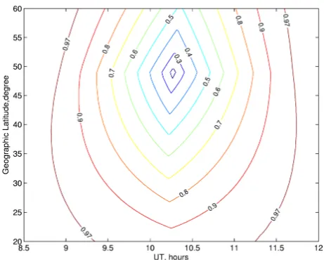
Figure 1. Contours of the revised eclipse factor, FR(UT, h, Φ, θ), as a function of universal time
564
(UT) and geographic latitude for an altitude of 200 km on the 1.67° E meridian during the solar 565
eclipse of August 11, 1999. 566
Fig. 1. Contours of the revised eclipse factor,FR(UT, h,8, θ ), as a function of universal time (UT) and geographic latitude for an altitude of 200 km in the 1.67◦E meridian during the solar eclipse of 11 August 1999.
24 -567
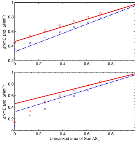
Figure 2. Scatterplots of ΔNmE (circles) and ΔNmF1 (crosses) versus ΔSp and a linear fit for
568
these observations (solid line for ΔNmE; dashed line for ΔNmF1). 569
570
Fig. 2. Scatterplots of1NmE (circles) and1NmF1 (crosses) versus
1Spand a linear fit for these observations (solid line for1NmE; dashed line for1NmF1).
eclipse event, which is in accord with the result of Davis et al. (2000). In this study, we define a revised eclipse factor FR(UT, h,8,θ )as the ratio of the unmasked solar radiation to the total solar radiation including the radiation originat-ing both in the photosphere and in the corona, which actually represents the percentage of the unmasked solar radiation at a given time (UT) and location (h,8,θ ). To calculate the value of theFR(UT, h,8,θ ), we first calculate the eclipse magni-tude at a given time and location by a JavaScript Eclipse Cal-culator, which is a java program developed by Chris O’Byrne and Stephen McCann with the open source code on the web site (http://www.chris.obyrne.com/Eclipses/calculator.html). When the eclipse magnitude at any moment and any loca-tion is known, according to the astronomical model of Curto et al. (2006), we can calculate theFR(UT, h, 8,θ ) at the corresponding time and location. Figure 1 illustrates the dis-tribution of the revised eclipse factorFR(UT, h,8,θ )at an altitude of 200 km in the 1.67◦E meridian as a function of UT and geographic latitude. As shown in Fig. 1, a total eclipse occurred at 48.9◦N with a percentage of 22% of the solar ra-diation emitted by the unmasked part of the solar corona at the eclipse totality, and there was a partial eclipse between 20◦N and 48.9◦N. For a partial eclipse, a maximum eclipse is the instant when the greatest fraction of the Sun’s diame-ter is occulted. For a total eclipse, maximum eclipse is the instant of mid-totality. From Fig. 1 one can find that around the time of UT=10.35 (10:21 UT), there occurs a maximum eclipse for all eclipse regions between 20◦N and 60◦N in the 1.67◦E meridian.
The simulation was carried out in a magnetic plane (np, nl) (np=201, nl=100), where np is the number of points along a magnetic field line,nlis the number of magnetic field lines, with a time step of 60 s. The geomagnetic longitude of the magnetic plane is 70◦E, the associated geographic longi-tude 1.67◦E. The geomagnetic latitude ranges from 55◦S to 55◦N. The following geophysical parameters on 11 August 1999 are adopted: F10.7=130.8, F10.7A=164.5, 3 h
geomag 25 geomag -571
Figure 3. Comparison of linear fit for the observed ΔNmE (solid line) and ΔNmF1 (dotted line) 572
which is the same as Figure 2 with the modelled ΔNmE (circles) and ΔNmF1 (crosses) by using 573
the revised eclipse factor FR (Top) and the unrevised eclipse factor F (Bottom), respectively.
574
Fig. 3. Comparison of linear fit for the observed1NmE (solid line) and1NmF1 (dotted line) which is the same as Fig. 2 with the mod-elled1NmE (circles) and1NmF1 (crosses) by using the revised eclipse factorFR(Top) and the unrevised eclipse factor F (Bottom), respectively.
netic indexAP=(12, 7, 3, 4, 4, 4, 9, 6). We run a simulation with the revised eclipse factor FR(UT, h, 8, θ )described above, with the results denoted by subscript E(on eclipse day). In order to identify the effects of the eclipse, a further simulation was run for identical conditions but excluding the eclipse shadow, with the results denoted by subscriptC(on control day). In addition, we run a simulation with the un-revised eclipse factorF(UT, h,8,θ )to compare the result with that of usingFR(UT, h,8,θ ).
4 Results and discussions
[image:4.595.52.287.65.198.2]1NmF1 is always smaller than1NmE from the figure. At totality (1SP=0), 1NmE falls to about 0.46 and 1NmF1 falls to about 0.32. Furthermore, for each ionosonde station which records both NmE and NmF1,1NmF1 is also smaller than1NmE. In conclusion, during an eclipse the relative re-sponse of the electron density in the F1 layer is greater than that in the E layer.
In Fig. 3, we plot the linear fit for the observations (as shown in Fig. 2) and the modeled1NmE and1NmF1. The modeled results from using the revised eclipse factor FRare plotted in the upper panel and the modelled results from using the unrevised eclipse factor F are plotted in the bot-tom panel. The seven modelled results plotted in Fig. 3 are for locations over 29.6◦N, 32.7◦N, 35.8◦N, 39.0◦N, 42.2◦N, 45.5◦N, and 48.9◦N, respectively, with the maxi-mum eclipse magnitude of 0.4, 0.5, 0.6, 0.7, 0.8, 0.9 and 1.0, respectively. From Fig. 3, one can find that the revised eclipse factorFRmakes the modelled results in accord with the measured results, whereas the unrevised eclipse factor F results in a large deviation between the modelled results and the measured ones. It can be concluded that, the revised eclipse factorFRis fairly accurate for the description of the variation in solar radiations. As shown in Fig. 3, the mod-elled results suggest that there is a larger decrease in NmF1 than in NmE, which is in accord with the measured results. A similar result was reported by Roble et al. (1986). Both measured and modelled results reveal that during the eclipse the response of electron density in the F1 layer is larger than that in the E layer.
It is now well known that the E and F1 region are mainly dominated by the photochemical process, so ionospheric pa-rameters NmE and NmF1 should be sensitive to changes in radiations caused by a solar eclipse. Both observations (as shown in Fig. 2) and calculations (as shown in Figs. 3 and 4) show that there are marked decreases in NmE and NmF1, though only a partial eclipse with a small eclipse magnitude occurred.
Given that the E-region behaves like anα-Chapman layer, the electron density in the E-region on the eclipse day and control day satisfies Eqs. (1) and (2), respectively:
dNeE
dt =FR·q0(χ )−α·Ne 2
E (1)
dNeC
dt =q0(χ )−α·Ne 2
C (2)
where NeE and NeC are the electron density on the eclipse day and control day,q0(χ )is the normal production rate,χ is the solar zenith angle,FR is the eclipse factor defined in Sect. 3, andαis the recombination rate coefficient. The so-lar eclipse is not a very rapid variation process; take the 11 August 1999 eclipse, for example, for a given place, such as 49.8◦N and 1.67◦E, it took more than three hours to cover the whole eclipse process from the eclipse begin to the eclipse end. So we can assume a quasi-stationary state for
26
[image:5.595.310.544.64.250.2]-575
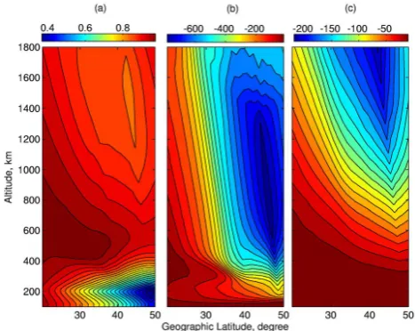
Figure 4. Contours of the relative change in electron density (a), NeE/NeC, electron temperature
576
(b), TeE – TeC, and ion O+ drift velocity along field line (positive upward) (c), ViOE – ViOC, as a
577
function of geographic latitude and altitude at 1021 UT. The longitude is about 1.67° E. These 578
results are calculated by the ionospheric model. 579
580
Fig. 4. Contours of the relative change in electron density (a),
NeE/NeC, electron temperature (b), TeE– TeC, and ion O+drift velocity along field line (positive upward) (c), ViOE–ViOC, as a function of geographic latitude and altitude at 10:21 UT. The lon-gitude is about 1.67◦E. These results are calculated by the iono-spheric model.
the eclipse that the left sides of the continuity Eqs. (1) and (2) become zero. Under the assumption of a quasi-stationary state, from Eqs. (1) and (2) we can obtain the relative de-crease in electron density1NmE=NeE/NeC=FR1/2. At total-ity, the FR reaches a minimum of about 0.22, so the mini-mum1NmE≈0.47. This value is consistent with both the result derived from the linear fit of the observations (about 0.46) and the modeling result (about 0.446).
The F1 region lies at a region of transition from the “square law” loss formula αN2 to the “linear” formula βN (Rat-cliffe, 1956; Rishbeth, 1968). If the F1-region is governed by a linear loss βN, the relative decrease in electron den-sity NeE/NeC is equal toFR, i.e. at totality the1NmF1 is 0.22 under the assumption of a linear lossβN. And if the F1-region is governed by a square low lossαN2, at totality the value of the1NmF1 would be 0.47. The square law loss αN2and the linear lossβN are equally important in the F1-region. Therefore, at totality the1NmF1 should be equal to a value between 0.22 and 0.47. The corresponding values of 1NmF1 derived from observations and calculations are 0.32 and 0.37, respectively, which agrees with the discussion above.
27
-581
Figure 5. The values of the hmF2 at 1021 UT on eclipse day (dashed circle line) and on control 582
day (solid square line) versus geographic latitude. 583
Fig. 5. The values of the hmF2 at 10:21 UT on eclipse day (dashed
circle line) and on control day (solid square line) versus geographic latitude.
400 km and the largest change with1Ne=0.343 is attained at an altitude of about 185 km over 48.8◦N; there is little response with1Ne larger than 0.9 in the altitude range of 400 km–800 km; and there is also an obvious decrease in electron density with1Ne≈0.85 at a higher altitude range of 1200 km–1800 km. From Fig. 4a, we can find that over all “eclipse” regions (from 20◦N to 60◦N) the largest change in electron density is in the range of 180–200 km (F1 region). In addition, the height of this largest change rises with de-creasing latitude from around 185 km over 50◦N to around 205 km over 25◦N. Calculations also show that, compared to the normal behavior on the control day, there is an in-crease in the peak height of the F2 layer, hmF2 (as shown in Fig. 5) over all regions at maximum eclipse. The greater the eclipse magnitude is, the larger the change in hmF2. For ex-ample, hmF2 at 33◦N (partial eclipse with the eclipse mag-nitude of 0.5) rises from about 305 km to 315 km and hmF2 at 50◦N (total eclipse) rises from about 270 km to 295 km. The similar results have been reported by Evans (1965b), Stubbe (1970), Salah et al. (1986), and Boitman et al. (1999). As shown in Fig. 4a, for the height range between 200 km and 400 km, the lower the height is, the larger the magnitude of the decrease in electron density, i.e. the decrease in elec-tron densities at altitudes below the hmF2 is greater than that at latitudes above the hmF2, which causes a change in the shape of the height profile of the electron density and a rise in hmF2.
Figure 4b shows an overall decrease in electron tempera-ture throughout the entire height range except the E-region (below 140 km). The largest decrease in electron tempera-ture occurs in the altitudes of 600–1000 km over about 46◦N and reaches more than 700 K, whereas there is little drop
[image:6.595.53.283.62.262.2]28 -584
Figure 6. The simulated ionospheric response to the solar eclipse at latitude of 48.8° N. Time 585
evolution of the relative change in electron density (a), NeE/NeC, electron temperature (b), TeE –
586
TeC, and ion O+ drift velocity along field line (positive upward) (c), ViOE – ViOC. Circles on the
587
x-axis indicate the time of the commencement, totality and end of solar eclipse, respectively. 588
589
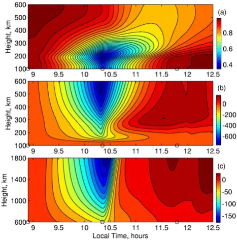
Fig. 6. The simulated ionospheric response to the solar eclipse at
latitude of 48.8◦N. Time evolution of the relative change in elec-tron density (a), NeE/NeC, elecelec-tron temperature (b), TeE–TeC, and ion O+ drift velocity along field line (positive upward) (c), ViOE– ViOC. Circles on the x-axis indicate the time of the commencement, totality and end of solar eclipse, respectively.
[image:6.595.310.544.65.304.2]in the topside ionosphere than at low heights (as shown in Fig. 4a). In addition, the downward ionization flux from the plasmasphere also leads to a decrease in electron density at this height (as shown in Fig. 4a).
4.2 Time-dependent response of the ionosphere to solar eclipse
As shown in Fig. 1, for 1.67◦E meridian, during the solar eclipse of 11 August 1999 the strongest eclipse occurred at about 49◦N. We plot time evolution of simulated ionospheric response to the solar eclipse in Fig. 6. Figure 6a shows the relative change in electron density1Ne, Fig. 6b shows the relative change in electron temperature1Te, and Fig. 6c shows the relative change in ion O+drift velocity1Vi (pos-itive upward) along the field line. From Fig. 6a, one can find that during the whole eclipse, eclipse effects on the electron density mainly occur at altitudes below 600 km. The time when a minimum of 1Ne is attained is height dependent. For altitudes below 200 km (the E- and F1-region) it is ap-proximately synchronous with the totality (about 10:21 UT), and at altitudes above 200 km it is markedly delayed with re-gard to the time of totality: the time lag between totality and the greatest reduction in Ne (corresponding minimum1Ne) increases with the altitude and reaches a maximum at about 600 km and then becomes smaller again. For example, the time lag is 15 min at 300 km, 60 min at 600 km, and 30 min at 1200 km, which is coincident with the results from Stubbe (1970). It is now well known that such a delay feature of the ionosphere is related to the “sluggishness” of the iono-sphere (Appleton, 1953; Rishbeth, 1968; Rishbeth and Gar-riott; 1969). It means that changes in Ne should theoretically lag behind changes in the electron production rate by a time constant of 1/2αN for the low altitudes and 1/βfor the high altitudes, whereαis the square law loss coefficient andβis the linear loss coefficient. Figure 6a also shows that before the totality the height of the1Ne minimum is at a constant altitude of about 200 km, whereas after that time it rises grad-ually with time. After totality the electron density at low heights begins to recover rapidly, whereas at high heights it still continues to decrease due to the time lag mentioned above, so the height of the1Ne minimum rises with time. Calculations also show that hmF2 rises with time, reaches a peak, and then decreases gradually to the usual daytime level at the end of the eclipse. The largest rise in hmF2 is about 25 km at 10:24 UT, i.e. the time delay of hmF2 response does not exceed 3 min.
Figure 6b presents the calculated height-time variation in 1Te during the eclipse. Calculations show that the begin-ning of the eclipse occurs simultaneously with an overall de-crease in electron temperature throughout the entire height range. At all heights changes in electron temperature are synchronous with the eclipse magnitude. The largest drop in electron temperature occurs at the time of totality. The typical value of1Te is about−200 K at 200 km,−500 K at
29
[image:7.595.312.544.66.251.2]-590
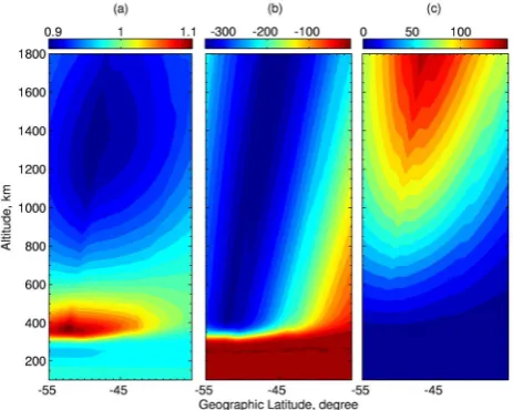
Figure 7. Same as Figure 4, but for the conjugate hemisphere (35° S – 55° S). 591
Fig. 7. Same as Fig. 4, but for the conjugate hemisphere (35◦S– 55◦S).
400 km, and−700 K at 600 km. After the totality the elec-tron temperature begins to increase gradually and recovers to the usual daytime level before the end of the eclipse. Further-more, calculations show that the electron temperature contin-ues to increase with the largest positive1Te of about 100 K, as shown in Fig. 6b, at the end of the eclipse. At this time, solar irradiation recovers to the usual level entirely; however, electron density is still relatively low, owing to recombina-tion, which causes a small increase in Te. These results are similar to the increase in Te at sunrise.
The height-time variation in the calculated ion drift veloc-ity difference 1Vi is shown in Fig. 6c. Due to a decrease in the diffusive equilibrium scale height which is caused by a decrease in electron and ion temperature, the ion in the higher altitudes moves downwards to make up for ion losses in the lower ionosphere. As shown in Fig. 6c, the largest ion flux downwards occurs at totality for all height ranges. With the recovery of electron density and temperature, the ion flux downwards decreases gradually. The lower ionosphere re-covers much faster than the upper ionosphere, which causes the downward velocity to diminish. Near the end of the eclipse, the ion drift velocity may even change its direction at higher altitudes due to the recovery of the electron density and the small increase in electron temperature.
value of1Ne≈0.9 at altitudes of 1200–1400 km, at the same time a small increase in electron density occurs in the F re-gion with the greatest increase value of1Ne≈1.1 at about 380 km. In the Northern Hemisphere the total eclipse occurs at about 49◦N, and its magnetic conjugate point is at 53◦S. So the associated greatest disturbance in the Southern Hemi-sphere should occur at 53◦S (as shown in Fig. 7a). Calcu-lations show that the greatest disturbance in electron density is delayed about 12 min compared to the time of maximum eclipse (10:21 UT). Figure 7b shows the there is an overall decrease in electron temperature at altitudes above 300 km in the conjugate hemisphere. The greatest decrease correspond-ing to the value of1Te≈350 K occurs in the region along geomagnetic field lines with the footpoints near 53◦S. Sim-ulations show that the greatest disturbance in electron tem-perature is almost synchronous, with the eclipse occurring in the Northern Hemisphere. As illustrated in Fig. 7c, there is an overall ion flux downward along the geomagnetic field line at altitudes above 400 km in the conjugate hemisphere.
Energetic photoelectrons are created during the photoion-ization of the neutral gases and heat the ambient electron gas. At lower altitudes, most of the photoelectron heat is distributed locally. At higher altitudes, the more ener-getic photoelectrons are able to propagate along the mag-netic field lines, heating the gas further afield with observ-able effects in the conjugate hemisphere (Millward et al., 1993). The phenomenon of the energetic photoelectron flow from a conjugate sunlit hemisphere to a darkness hemisphere has been mentioned and considered in some papers in the past (e.g. Evans, 1973; Schunk and Nagy, 1978; Bailey and Sellek, 1990; Chao et al., 2003, Zhang et al., 2004; Lei et al., 2007; Bilitza et al., 2007). When the North-ern Hemisphere is in darkness during the eclipse, the mag-netic conjugate-points in the Southern Hemisphere are still illuminated. The sunlit asymmetry between the two hemi-spheres causes an asymmetry of the distribution of photo-electron in the two hemispheres. Due to the decrease in solar radiations, the photoelectron production rate in the Northern Hemisphere decreases by a large magnitude at eclipse total-ity, which therefore causes a corresponding decrease in the photoelectron travelling along the magnetic field lines to the Southern Hemisphere and the heating of electron gas there. So at higher altitudes in the Southern Hemisphere, the elec-tron heating rate would decrease due to the large decrease in the photoelectron heating from the Northern Hemisphere, which causes a decrease in electron temperature, as shown in Fig. 7b. At lower altitudes in the Southern Hemisphere, the electron temperature is not affected during the eclipse pro-cess at the Northern Hemisphere, since the local heating ef-fect occurs at lower altitudes. For the Southern Hemisphere, the decrease in electron temperature causes a correspond-ing decrease in the scale height of plasma, which makes a redistribution of plasma and leads to a plasma flow down-ward along the geomagnetic field line (as shown in Fig. 7c), and therefore a small decrease in electron density in the
plasmasphere and a small increase in electron density in the F region (as shown in Fig. 7a).
Given the variable nature of the F region, a small increase in electron densities by only∼10% is hard to observe and therefore to validate. As for the 11 August 1999 solar eclipse event, its path of totality passing over central Europe, the conjugate hemisphere therefore locates over the southern At-lantic Ocean where there are no ionospheric observatories at all. As is known, there are far more ionospheric observato-ries in the Northern Hemisphere than in the southern hemi-sphere. For a solar eclipse event in the Southern Hemisphere, it might be possible to obtain more ionospheric data in the conjugate hemisphere and test this prediction. Given enough ionospheric stations worldwide, it might be possible to make the results statistically significant and we will continue to do relevant work later.
5 Summary
Using the data from 16 ionosonde stations in Europe, we per-form a statistical analysis of the response of the E- and F1-region to the 11 August 1999 eclipse. Then according to the astronomical model of Curto et al. (2006), we construct a re-vised eclipse factorFR(UT, h,8,θ ), which is equal to the ratio of the unmasked solar radiation to the total solar radi-ation, taking account of the radiation from the solar corona when calculating the total solar radiation. A middle and low latitude theoretical ionospheric model and the eclipse fac-torFR are used to model the ionospheric response to this eclipse. Both the observations and the calculations show that for the mid- and low latitude ionosphere, the decrease in the electron density during a solar eclipse is greater in the F1-region than in the E-F1-region. The simulations show that ex-cept the obvious ionospheric response at low altitudes below 500 km, there is also a small response at high altitudes up to about 2000 km. In addition, calculations show that when the eclipse takes place in the Northern Hemisphere there is also a small ionospheric disturbance in the conjugate hemisphere. The main simulated results are summarized as follows:
1. For the mid- and low latitude ionosphere, the decrease in the electron density during solar eclipse is greater in the F1 region than in the E region. The electron density at the altitude range of 1500–1800 km also decreases slightly. The eclipse also causes a marked drop in elec-tron temperature at altitudes above 200 km, with the largest drop of about 700 K in the topside ionosphere, while the ion temperature decreases slightly.
synchronous with the eclipse function, and it begins to increase at 30 min after the totality and reaches the largest value of about 200 K at the end of eclipse. 3. For the conjugated hemisphere, the electron density
de-creases slightly in the latitudes of 300–500 km and in-creases slightly in the latitudes of 1200–1600 km, and there is also an overall decrease in electron temperature with the largest value of about 300 K.
Acknowledgements. The authors wish to thank the Space Physics Interactive Data Resource of the National Geophysical Data Center for the supply of the ionospheric data. This research was supported by National Natural Science Foundation of China (40725014, 40674090, 40636032) and National Important Basic Research Project (2006CB806306).
Topical Editor M. Pinnock thanks C. J. Davis and another anonymous referee for their help in evaluating this paper.
References
Adeniyi, J. O., Radicella, S. M., Adimula, I. A., Willoughby, A. A., Oladipo, O. A., and Olawepo, O.: Signature of the 29 March 2006 eclipse on the ionosphere over an equatorial station, J. Geo-phys. Res., 112, A06314, doi:10.1029/2006JA012197, 2007. Afraimovich, E. L., Palamartchouk, K. S., Perevalova, N. P.,
Chemukhov, V. V., Lukhnev, A. V., and Zalutsky, V. T.: Iono-spheric effects of the solar eclipse of March 9, 1997, as deduced from GPS data, Geophys. Res. Lett., 25(4), 465–468, 1998. Afraimovich, E. L., Kosogorov, E. A., and Lesyuta, O. S.: Effects
of the August 11, 1999 total solar eclipse as deduced from total electron content measurements at the GPS network, J. Atmos. Sol.-Terr. Phy., 64, 1933–1941, 2002.
Appleton, E. V.: A note on the “sluggishness” of ionosphere, J. Atmos. Terr. Phys., 3, 228–232, 1953.
Bailey, G. J. and Sellek, R. A.: Mathematical model of the Earth’s plasmasphere and its application in a study of He+ at L = 3.0, Ann. Geophys., 8, 171–190, 1990,
http://www.ann-geophys.net/8/171/1990/.
Baran, L. W., Ephishov, I. I., Shagimuratov, I. I., Ivanov, V. P., and Lagovsky, A. F.: The response of the ionospheric total electron content to the solar eclipse on August 11, 1999, Adv. Space Res., 31(4), 989–994, 2003.
Bilitza, D., Truhlik, V., Richards, P., Abe, T., and Triskova, L.: Solar cycle variations of mid-latitude electron density and temperature: Satellite measurements and model calculations, Adv. Space Res., 39, 779–789, 2007.
Boitman, O. N., Kalikhman, A. D., and Tashchilin, A. V.: The midlatitude ionosphere during the total solar eclipse of March 9, 1997, J. Geophys. Res., 104(A12), 28 197–28 206, 1999. Chao, C. K., Su, S.-Y., and Yeh, H. C.: Presunrise
ion temperature enhancement observed at 600 km low and mid-latitude ionosphere, Geophys. Res. Lett., 30(4), 1187, doi:10.1029/2002GL016268, 2003.
Cheng, K., Huang, Y.-N., and Chen, S.-W.: Ionospheric effects of the solar eclipse of September 23, 1987, around the equatorial anomaly crest region, J. Geophys. Res., 97(A1), 103–111, 1992.
Cohen, E. A.: The study of the effect of solar eclipses on the iono-sphere based on satellite beacon observations, Radio Sci., 19, 3, 769–777, 1984.
Curto, J. J., Heilig, B., and Pinol, M.: Modeling the geomagnetic ef-fects caused by the solar eclipse of 11 August 1999, J. Geophys. Res., 111, A07312, doi:10.1029/2005JA011499, 2006.
Davis, C. J., Lockwood, M., Bell, S. A., Smith, J. A., and Clarke, E. M.: Ionospheric measurements of relative coronal brightness during the total solar eclipses of 11 August, 1999 and 9 July, 1945, Ann. Geophys., 18, 182–190, 2000,
http://www.ann-geophys.net/18/182/2000/.
Davis, C. J., Clarke, E. M., Bamford, R. A., Lockwood, M., and Bell, S. A.: Long term changes in EUV and X-ray emissions from the solar corona and chromosphere as measured by the re-sponse of the Earth’s ionosphere during total solar eclipses from 1932 to 1999, Ann. Geophys., 19, 263–273, 2001,
http://www.ann-geophys.net/19/263/2001/.
Evans, J. V.: An F Region Eclipse, J. Geophys. Res., 70, 131–142, 1965a.
Evans, J. V.: On the Behavior of foF2 during Solar Eclipses, J. Geophys. Res., 70, 733–738, 1965b.
Evans, J. V.: Seasonal and sunspot cycle variation of F region elec-tron temperatures and protonospheric heat flux, J. Geophys. Res., 78, 2344–2349, 1973.
Farges, T., Jodogne, J. C., Bamford, R., Roux Y. Le., Gauthier, F., Vila, P. M., Altadill, D., Sole, J. G., and Miro, G.: Disturbances of the western European ionosphere during the total solar eclipse of 11 August 1999 measured by a wide ionosonde and radar net-work, J. Atmos. Sol.-Terr. Phy., 63, 915–924, 2001.
Farges, T., Pichon, A. Le, Blanc, E., Perez, S., and Alcoverro, B.: Response of the lower atmosphere and the ionosphere to the eclipse of August 11, 1999, J. Atmos. Sol.-Terr. Phy., 65, 717– 726, 2003.
Hedin, A. E., Fleming, E. L., Manson, A. H., et al.: Empirical wind model for the upper, middle and lower atmosphere, J. Atmos. Terr. Phys., 58, 1421–1447, 1996.
Huang, C. R., Liu, C. H., Yeh, K. C., Lin, K. H., Tsai, W. H., Yeh, H. C., and Liu, J. Y.: A study of tomographically recon-structed ionospheric images during a solar eclipse, J. Geophys. Res., 104(A1), 79–94, 1999.
Hunter A. N., Holman, B. K., fieldgate, D. G., and Kelleher, R.: Faraday rotation studies in Africa during the solar eclipse of June 30, 1973, Nature, 250, 205–206, 1974.
Klobuchar, J. A. and Whitney, H. E.: Ionospheric electron content measurements during a solar Eclipse, J. Geophys. Res., 70(5), 1254–1257, 1965.
Korenkov, Y. N., Klimenko, V. V., Baran, V., Shagimuratov, I. I., and Bessarab, F. S.: model calculations of TEC over Europe dur-ing 11 August 1999 solar eclipse, Adv. Space Res., 31(4), 983– 988, 2003a.
Korenkov, Y. N., Klimenko, V. V., Bessarab, F. S., Nutsvalyan, N. S., and Stanislawska, I.: Model/data comparison of the F2-region parameters for the 11 August 1999 solar eclipse, Adv. Space Res., 31(4), 995–1000, 2003b.
Lei, J., Liu, L., Wan, W., and Zhang, S. R.: Modeling the behavior of ionosphere above Millstone Hill during the September 21-27, 1998 storm, J. Atmos. Sol.-Terr. Phy., 66, 1093–1102, 2004a. Lei, J., Liu, L., Wan, W., and Zhang, S. R.: Model results for the
Geo-phys., 22, 2037–2045, 2004b.
Lei, J.: Statistical analysis and modeling investigation of middle latitude ionosphere. Dissertation for the Doctoral Degree. Bei-jing: Institute of Geology and Geophysics, Chinese Academy of Sciences, 2005.
Lei, J., Roble, R. G., Wang, W., Emery, B. A., and Zhang, S.-R.: Electron temperature climatology at Millstone Hill and Arecibo, J. Geophys. Res., 112, A02302, doi:10.1029/2006JA012041, 2007.
Liu, L., Wan, W., Tu, J. N., Bao, Z. T., and Yeh, C. K.: Model-ing study of the ionospheric effects durModel-ing a total solar eclipse, Chinese J. Geophys, 42(3), 296–302, 1999.
Millward, G. H.: A global model of the earth’s thermosphere, iono-sphere and plasmaiono-sphere: theoretical studies of the response to enhanced high-latitude convection, Dissertation for the Doctoral Degree, UK: University of Sheffield, 1–195, 1993.
M¨uller-Wodarg, I. C. F., Aylward, A. D., and Lockwood, M.: Ef-fects of a Mid-Latitude Solar Eclipse on the Thermosphere and Ionosphere – A Modelling Study, Geophys. Res. Lett., 25(20), 3787–3790, 1998.
Oliver, W. L. and Bowhill, S. A.: The F1 region during a solar eclipse, Radio. Sci., 9(2), 185–195, 1974.
Picone, J. M., Hedin, A. E., Drob, D. P., and Aikin, A. C.: NRLMSISE-00 empirical model of the atmosphere: statistical comparisons and scienti5c issues, J. Geophys. Res., 107(A12), 1468, doi:10.1029/2002JA009430, 2002.
Ratcliffe, J. A.: The formation of the ionospheric layers F1 and F2, J. Atmos. Terr. Phys., 8, 260–269, 1956.
Richards, P. G., Fennelly, J. A., and Torr, D. G.: EUVAC: A Solar EUV Flux Model for Aeronomic Calculations, J. Geophys. Res., 99, 8981–8992, 1994.
Rishbeth, H.: Solar eclipses and ionospheric theory, Space. Sci. Rev., 8(4), 543–554, 1968.
Rishbeth, H. and Garriott, O. K.: Introduction to Ionospheric Physics, Academic Press, San Diego, CA, 1969.
Roble, R. G., Emery, B. A., and Ridley, E. C.: Ionospheric and Thermispheric Response Over Millstone Hill to the May 30, 1984, Annular Solar Eclipse, J. Geophys. Res., 91(A2), 1661– 1670, 1986.
Salah, J. E., Oliver, W. L., Foster, J. C., and Holt, J. M.: Observa-tions of the May 30, 1984, Annular Solar Eclipse at Millstone Hill, J. Geophys. Res., 91(A2), 1651–1660, 1986.
Schunk, R. W. and Nagy, A. F.: Electron temperatures in the F re-gion ionosphere: Theory and observations, Rev. Geophys., 16, 355–399, 1978.
Stubbe, P.: The F-region during an eclipse – A theoretical study, J. Geophys. Res., 32, 1109–1116, 1970.
Titheridge, J. E.: Model results for the ionospheric E-region: solar and seasonal changes, Ann. Geophys., 15, 63–78, 1997, http://www.ann-geophys.net/15/63/1997/.
Tom´as, A. T., L¨uhr, H., F¨orster, M., Rentz, S., and Rother, M.: Observations of the low-latitude solar eclipse on 8 April 2005 by CHAMP, J. Geophys. Res., 112, A06303, doi:10.1029/2006JA012168, 2007.
Tsai, H. F. and Liu, J. Y.: Ionospheric total electron content re-sponse to solar eclipses, J. Geophys. Res., 104(A6), 12 657– 12 668, 1999.
Tu, J. N., Liu, L., and Bao, Z. T.: An low latitude theoretical iono-spheric model, Chinese J. Space Sci (in Chinese), 17, 212–219, 1997.
Yue, X., Wan, W., Liu, L., Le, H., Chen, Y., and Yu, T.: Develop-ment of a middle and low latitude theoretical ionospheric model and an observation system data assimilation experiment, Chinese Sci. Bull., 53(1), 94–101, 2008.