Thrust calculation of electric solar wind sail by particle-in-cell simulation

www.ann-geophys.net/34/845/2016/ doi:10.5194/angeo-34-845-2016

© Author(s) 2016. CC Attribution 3.0 License.

Thrust calculation of electric solar wind sail by

particle-in-cell simulation

Kento Hoshi1, Hirotsugu Kojima2, Takanobu Muranaka3, and Hiroshi Yamakawa2

1_{Department of Electrical Engineering, Graduate School of Engineering, Kyoto University, Kyoto, Japan} 2_{Research Institute for Sustainable Humanosphere, Kyoto University, Kyoto, Japan}

3_{Department of Electrical Engineering, Chukyo University, Nagoya, Japan}

Correspondence to:Kento Hoshi ([email protected])

Received: 1 July 2016 – Revised: 25 August 2016 – Accepted: 7 September 2016 – Published: 26 September 2016

Abstract. In this study, thrust characteristics of an electric solar wind sail were numerically evaluated using full three-dimensional particle-in-cell (PIC) simulation. The thrust ob-tained from the PIC simulation was lower than the thrust es-timations obtained in previous studies. The PIC simulation indicated that ambient electrons strongly shield the electro-static potential of the tether of the sail, and the strong shield effect causes a greater thrust reduction than has been ob-tained in previous studies. Additionally, previous expressions of the thrust estimation were modified by using the shielded potential structure derived from the present simulation re-sults. The modified thrust estimation agreed very well with the thrust obtained from the PIC simulation.

Keywords. General or miscellaneous (instruments useful in three or more fields; new fields (not classifiable under other headings); techniques applicable in three or more fields)

1 Introduction

An electric solar wind sail, called the “E-sail,” is a recently proposed propulsion device that consists of 50–100 conduc-tive tethers with lengths of 10–20 km and thicknesses of 0.1– 1 µm. The E-sail was first proposed by Janhunen (2004). The main body of the spacecraft expands the tethers to form a sail-like structure. The E-sail has electron guns to maintain a positive surface potential on the order of several kilovolts, in order to deflect solar wind protons. The tethers obtain the momentum of these deflected protons via Coulomb scatter-ing and use it as their propulsive force. The system requires electron sources and electrical power for the electron guns to

produce thrust. The E-sail is expected to be used as a new propellantless space propulsion device.

The thrust characteristics of the E-sail were first investi-gated by Janhunen and Sandroos (2007). They performed a one-dimensional (1-D) particle-in-cell (PIC) simulation of a conductive tether with a radius of 1.0 m. They found that an ansatz of the electrostatic potential structure around the tether, which is expressed as

V (r)=V0

2 ln

1+(2λD/r)2 ln(2λD/rw)

, (1)

agreed very well with the result of their PIC simulation, whereris the distance from the tether,V0is the surface po-tential of the tether,λD=

p

ε0kBTe/e2neis the Debye length of the electron, andrwis the radius of the tether. For

evaluat-ing the performance of an E-sail, the thrust per unit length is often used. The total thrust can be calculated from the thrust per unit length by multiplying the number of tethers by the length of one tether. Janhunen and Sandroos (2007) also conducted a two-dimensional (2-D) PIC simulation and suggested that the thrust per unit length acting on the tether is

dF

dL =

Kmpn0v2_dr0

s

exp

mpvd2

eV0 ln(

r0

rw)

−1

, (2)

may increase because of a lack of electrons around the tether. He proposed the use of multiple tethers to collect ambient electrons so that the electron density around each tether de-creases and the ambient electrons cannot completely shield the potential of the tether. According to Janhunen (2009), the thrust with ambient electron removal is 5 times larger than that obtained by Janhunen and Sandroos (2007) without am-bient electron removal.

Sanchez-Torres (2014) also investigated the thrust of the E-sail considering Coulomb scattering, assuming the absence of trapped electrons around the tether. He expressed the po-tential structure as

V (r)=V0



  

  

ln

rshe−b

r

ln

r_she−b

rw

(r≤rshe

−b₎

0 (r > rshe−b)

, (3)

where the approximated parameterb is 0.65 for a potential bias ofV0=10–40 kV andrshis the sheath radius for a highly positive bias tether and can be calculated from the ambient plasma parameters andV0(Sanmartín et al., 2008). Using the solar wind parameters at 1 AU, the thrust per unit length is 407 nN m−1for a 20 kV charged tether ofrw=20 µm. This is

lower than the thrust per unit length of 500 nN m−1estimated by Janhunen (2009) but higher than the value of 100 nN m−1 estimated by Janhunen and Sandroos (2007) because Eq. (3) yields greater values of the potential than Eq.(1) under al-most all conditions. The study by Sanchez-Torres (2014) was purely analytical; no plasma simulations were performed.

However, Hoshi et al. (2016) showed that the actual elec-trostatic potential structure around the tether was lower than those given by Eqs. (1) and (3) based on the results of a full three-dimensional (3-D) PIC simulation with V0=240 V. The thrust of the E-sail is generated from the deflection of solar wind protons by the electrostatic potential. If the elec-trostatic potential derived from the tethers is greatly shielded by ambient electrons, the actual thrust is lower than that es-timated in previous studies. Hoshi et al. (2016) did not con-sider the thrust because a potential of 240 V was not suffi-cient to deflect solar wind protons with a drift velocity of approximately 400 km s−1(≈0.8 keV).

In the present paper, we performed 3-D full PIC simula-tions to simulate a transient of the thrust of the E-sail. The thrust found in this paper is lower than that obtained in pre-vious studies, with a sufficiently high potential to deflect am-bient protons (V0>1 kV). Section 2 discusses the 3-D PIC simulation withV0≤4.0 kV that was performed to confirm that the potential was lower than those obtained from Eqs. (1) and (3). The propulsive force that acts on the tether is also calculated in the PIC simulation. In Sect. 3, the thrust is nu-merically estimated and compared with the PIC results. Two estimation procedures employed in previous studies (Jan-hunen and Sandroos, 2007; Sanchez-Torres, 2014) are modi-fied to contain a shielded potential structure derived from the

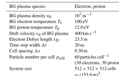
Table 1.Simulation parameters (BG: background).

BG plasma species Electron, proton

BG plasma densityn0 107m−3

BG electron temperatureTe 100 eV

BG proton temperatureTp 12.0 eV

Drift velocityvdof BG plasma 400 km s−1

Electron Debye lengthλD 23.5 m

Time step width1t 20 ns

Cell spacing1x 0.30 m

Particle number per cellpcell 60 particles cell−1

(30 electrons, 30 protons)

System size 512×512×512 cells

=(153.6 m)3

present simulation results. The estimated thrust and the PIC results are found to be in good agreement with each other and lower than those estimated in previous studies.

2 Full PIC simulation of E-sail 2.1 Simulation settings

This section describes the PIC simulation configurations of a positively charged tether in the solar wind environment. The simulation code HiPIC, which was developed by the Japan Aerospace Exploration Agency’s Engineering Digital Innovation Center (JEDI) (Muranaka et al., 2011), was used to perform this simulation. HiPIC is an electrostatic code that models 3-D rectangular cells in space and uses the full PIC method to calculate collisionless kinetic plasma. HiPIC solves Newton’s equations of motion for each particle us-ing the Buneman–Boris method and solves Poisson’s equa-tions to obtain the electric potential structure in the compu-tational domain using a discrete sine transformation. HiPIC can be used to calculate the interaction between plasmas and the spacecraft, which is modeled with rectangular internal boundaries. A detailed description of the performance of the code is given in Muranaka et al. (2011).

The simulation and physical parameters are given in Ta-ble 1. The electron density ne and the proton density np arene=np=n0=1.0×107m−3, and their temperatures are

kBTe=100 eV and kBTp=12 eV, respectively. The back-ground plasmas have a solar wind drift velocity of vd= 400 km s−1along thex axis. All of the edges of the simula-tion domain were fixed toV =0V (Dirichlet boundary con-dition). The background plasma particles were injected from all the domain boundaries in each time step as many times as the number of outgoing particles in previous time step.

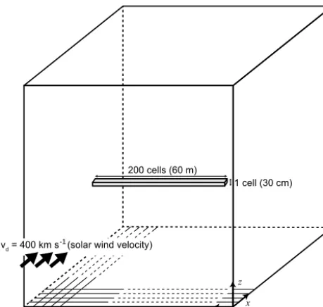
1 cell (30 cm) 200 cells (60 m)

Δx = 30 cm

vd = 400 kms (solar wind velocity)

x y

z -1

Figure 1.Definition of the tether model. A tether-like rectangle is located in the center of the computational domain. The solar wind originates fromx=0.

30 and 75 m were also simulated to confirm the influence of the length of the tether on the thrust per unit length.

Because of the limitation of the calculation resources, we cannot include the emission of the electron beam from the tether’s edge and simulate the self-charging of the tether. In-stead of emitting the electron, the surface potentialV0of the tether was fixed to an inputted value. Hoshi et al. (2016) showed that effects of emitted electrons on the potential structure were small, so we consider that the absence of emit-ted electrons do not cause significant differences in the force acting on the tether.

V0was varied from 0 to 4.0 kV, and the thrust acting on the tether Fx was calculated. Fx is thex component of the

thrust and was calculated as the sum of the total momentum of the particles impinging on the tether during each time step divided by 1t and the Coulomb force calculated from the Maxwell stress tensor. The simulation progressed with time steps of 1t=20 ns until the time variation of the external force became zero. In almost all the cases, the total iteration was 10 000 steps (=0.2 ms). An additional 2000 steps were calculated for theV0=4.0 kV case.

To perform the computation, we applied an MPI paral-lelization and an OpenMP paralparal-lelization. Each case used 2048 cores on Cray XE4 for calculation (1024 processes for MPI, two threads for OpenMP), requiring approximately 12 h to run.

2.2 Simulation results

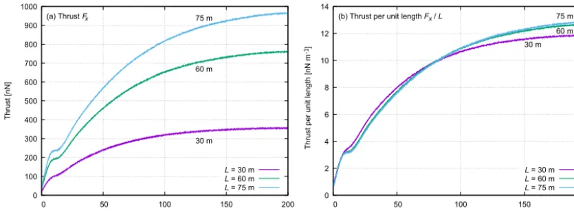
Figure 2a shows the time variation ofFxatV0=1.3 kV. At the beginning of the simulation,Fxwas almost zero because

the ambient particles had not yet begun to respond to the elec-trostatic potential of the tether.Fx then increased with time

and converged to a specific value. At the end of the simu-lation,Fx was 0.35, 0.76, and 0.96 µN forL=30, 60, and

75 m, respectively. These values represent the total force act-ing on the tether, includact-ing the sum of the particles hittact-ing the whole tether and the force calculated from the Maxwell stress tensor. However, the thrust per unit length indicates the performance of the E-sail; thus,Fx/Lwas calculated, as

shown in Fig. 2b.Fx/Lwas 11.7, 12.7, and 12.8 nN m−1for L=30, 60, and 75 m, respectively. The thrust per unit length forL=30 m was slightly smaller than that for 60 and 75 m. This lower value ofFx/L may be due to the end effect or

the effect which arises whenLis small in comparison with

λD. At L=60 and 75 m, the values of Fx/L were almost

equal; thus,L=60 m is considered to be sufficiently long to simulate an infinite tether.

The kinks in the thrust betweent=10 and 20 µs shown in Fig. 2 correspond to collections of ambient electrons. Fig-ure 3 shows the time history of the current on the surface of the tether withL=60 m. The ambient electron current (pur-ple line) varied dramatically betweent=10 and 20 µs. This is an initial response of the ambient electrons to the poten-tial of the tether. The electron plasma frequencyωpwas ap-proximately 178 kHz so the response time of ambient elec-trons were approximately 5.6 µs. Collected elecelec-trons do not directly contribute to the thrust, because their momentum is small. Instead, they temporarily shield the potential structure more strongly than in a steady state, causing the thrust to stop increasing with time, as shown in Fig. 2.

Figure 3 also reveals that the dominant source of the force acting on the tether was the force from the Maxwell stress tensor, not from the protons hitting the tether because the pro-ton current was almost zero. This fact shows that the compu-tation successfully simulates the thrust generation by proton deflection.

To compare the present results with previous thrust es-timations, Fx/L was calculated at various V0 values, as shown in Fig. 4. The blue line in Fig. 4 is the result of our PIC simulation withL=60 m and rw=15 cm. The black

and red dotted lines show the thrust estimated by Janhunen and Sandroos (2007) and Sanchez-Torres (2014), respec-tively, withrw=15 cm. In the present simulation,Fx/Lwas

67.1 nN m−1atV0=4.0 kV; in contrast, Janhunen and San-droos (2007) and Sanchez-Torres (2014) estimatedFx/Lto

be 123 and 246 nN m−1, respectively. These results indicate that the thrust characteristics of the E-sail are different from those of conventional estimations. This difference is likely due to the difference in the potential structure around the tether.

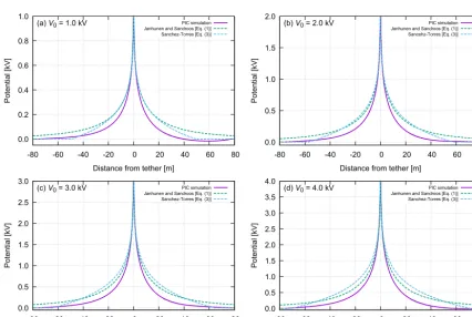
Figure 5 compares the electrostatic potential structures obtained in the present study and two previous studies at

0 100 200 300 400 500 600 700 800 900 1000

0 50 100 150 200

a) Thrust

30 m 60 m 75 m

Thrust [nN]

Time [µs]

L = 30 m L = 60 m L = 75 m

0 2 4 6 8 10 12 14

0 50 100 150 200

b) Thrust per unit length Fx / L

30 m 60 m 75 m

Thrust per unit length [nN

P

]

Time [µs]

L = 30 m L = 60 m L = 75 m Fx

-1

Figure 2.Time history of the thrust withV0=1.3 kV:(a)xcomponent of the total external force;(b)xcomponent of the thrust per unit

length.

-2.0 -1.8 -1.6 -1.4 -1.2 -1.0 -0.8 -0.6 -0.4 -0.2 0.0 0.2

0 50 100 150 200

Electron current

Proton current

Current [mA]

Time [µs]

Electron (L = 60 m)

Proton (L = 60 m)

Figure 3.Time history of the ambient electron and proton currents (V0=1.3 kV,L=60 m).

tained from the present PIC simulations was lower than the potentials obtained using Eqs. (1) and (3). Figure 5 indicates that potential shielding by ambient electrons is not appropri-ately included in Eqs. (1) and (3). Figure 5 also shows that the sheath length assumed by Eq. (3) is consistent with that obtained by PIC simulation.

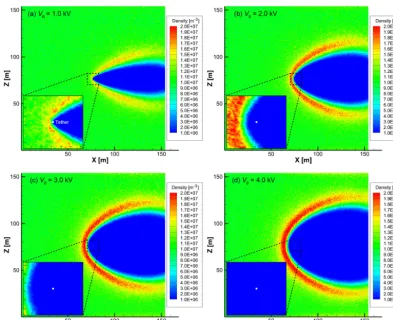
Figure 6 shows the proton density structure att=0.2 ms. AtV0=2.0, 3.0, and 4.0 kV, a zero-density (np=0 m−3) re-gion was present in front of the tether. No protons impinged on the surface of the tether. The momentum of the protons was transferred to the tether through the Coulomb force act-ing on the tether. In contrast, there was no zero-density re-gion in front of the tether atV0=1.0 kV. This is because the radiusrw of the tether is relatively large. The drift velocity

of the proton (400 km s−1) is equivalent to 0.83keV, but the figure indicates thatV0=1.0 kV is not sufficient to deflect all of the protons forrw=15 cm. Although a wake region is

present atV0=1.0 kV, it was formed by protons impinging on the surface of the tether. At a very smallrw, a zero-density

region may appear forV0=1.0 kV.

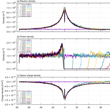
This study then considered the high-density proton region in front of the tether. Figure 7 shows the electron and pro-ton density structure along the x axis at V0=2.0 kV. As with Fig. 3a in Janhunen and Sandroos (2007), Fig. 7b re-veals a high-density region in front of the tether. The maxi-mum proton density was 2.0×107m−3atV0=2.0 kV. The maximum electron density was approximately 1.0×108m−3 at V0=2.0 kV. The maximum positive charge density of the high-density region is one fifth of the negative charge density of the electrons. The high-density region does not compensate for the potential; that is, it does not reduce the shielding effect of the electrons. Trapped electron removal, which was discussed by Janhunen (2009), was not observed in the present simulation. Thus, the thrust models given by Eqs. (1) and (3) are inappropriate for estimating the thrust of the E-sail, and a new model considering appropriate potential shielding must be developed.

0 20 40 60 80 100 120 140

0.5 1.0 1.5 2.0 2.5 3.0 3.5 4.0

Estimated thrust per unit length [nN

P

]

Potential [kV]

PIC simulation Janhunen and Sandroos 2007

Sanchez-Torres 2014

Janhunen and Sandroos (2007) Sanchez-Torres (2014)

PIC simulation

-1

Figure 4.Comparison of present thrust simulation results with previous estimations. The blue line shows the thrust obtained from the present PIC simulation withL=60 m andrw=15 cm. The black and red dashed lines show the thrust estimated by Janhunen and Sandroos (2007)

and Sanchez-Torres (2014), respectively, withrw=15 cm. The estimation procedures used in these two previous studies are described in

Sect. 3.

0.0 0.2 0.4 0.6 0.8 1.0

-80 -60 -40 -20 0 20 40 60 80

(a) V0 = 1.0 kV

Potential [kV]

Distance from tether [m] PIC simulation Janhunen and Sandroos [Eq. (1)] Sanchez-Torres [Eq. (3)]

0.0 0.5 1.0 1.5 2.0

-80 -60 -40 -20 0 20 40 60 80

(b) V0 = 2.0 kV

Potential [kV]

Distance from tether [m] PIC simulation Janhunen and Sandroos [Eq. (1)] Sancehz-Torres [Eq. (3)]

0.0 0.5 1.0 1.5 2.0 2.5 3.0

-80 -60 -40 -20 0 20 40 60 80

(c) V0 = 3.0 kV

Potential [kV]

Distance from tether [m] PIC simulation Janhunen and Sandroos [Eq. (1)] Sanchez-Torres [Eq. (3)]

0.0 0.5 1.0 1.5 2.0 2.5 3.0 3.5 4.0

-80 -60 -40 -20 0 20 40 60 80

(d) V0 = 4.0 kV

Potential [kV]

Distance from tether [m] PIC simulation Janhunen and Sandroos [Eq. (1)] Sanchez-Torres [Eq. (3)]

Figure 6.Proton density structure at the center of the tether (y=76.8 m) at tether surface potentials of(a)V0=1.0 kV,(b)V0=2.0 kV,

(c)V0=3.0 kV, and(d)V0=4.0 kV. The ambient plasma conditions aren0=10 cm−3,Te=100 eV, andTp=12 eV.

the realistic electrostatic potential given by the 2-D FFT. The thrust estimation script written by Python 2.7 is found in the Supplement (available online).

3.1 Semi-analytical solver of electrostatic potential structure

The Poisson equation in plasma is expressed as

∇2V (r)= −ρ(r) ε0

− e ε0

np(r)−ne(r)

, (4)

whereρ is the space charge density. From the velocity dis-tribution function of electrons, we assume that the electron’s density distribution becomes the Boltzmann distribution:

ne(r)=n0exp

eV (r) kBTe

. (5)

Assuming that the normalized potential eV (r)/kBTe be-comes small in the distance and also assuming thatnp=n0, Eq. (4) becomes

∇2V (r)= −ρ(r) ε0

+ e

2_n 0

ε0kBTe

V (r) (6)

with the first-order approximation. Defining kD=

e2n0/ε0kBTe, we obtain

(∇2−k2_D)V (r)= −ρ(r) ε0

. (7)

The 1-D solution of Eq. (7) is well known and is called the Yukawa potential. However, the 2-D analytical solution of Eq. (7), which would represent the shielded potential struc-ture around an infinite tether, remains unknown. This is why previous studies had to assume an artificial potential struc-ture, such as those given by Eqs. (1) and (3).

Hoshi et al. (2016) developed a numerical method of cal-culating the potential structure around a tether in plasma, adding the termh2k_D2 to the solution of the difference equa-tion corresponding to the differential equaequa-tion given by Eq. (7) as follows

Vm, n= h2 ε0

ρm, n

4+h2_k2

D−Wm−W−m−Wn−W−n

,

W=e2π i/N, (8)

whereVm, nis the electrostatic potential solution inkspace

0.0 × 100 2.0 × 107 4.0 × 107 6.0 × 107 8.0 × 107 1.0 × 108

1.2 × 108 (a) Electron density

Density [m

-3]

t = 0 µs t = 25 µs t = 50 µs t = 75 µs t = 100 µs t = 125 µs t = 150 µs t = 175 µs t = 200 µs

0.0 × 100 5.0 × 106 1.0 × 107 1.5 × 107 2.0 × 107

(b) Proton density

Density [m

-3]

t = 0 µs t = 25 µs t = 50 µs t = 75 µs t = 100 µs t = 125 µs t = 150 µs t = 175 µs t = 200 µs

-2.0 × 10-11 -1.6 × 10-11 -1.2 × 10-11 -8.0 × 10-12 -4.0 × 10-12 0.0 × 100 4.0 × 10-12

-80 -60 -40 -20 0 20 40 60 80

(c) Space charge density

Charge density [C/m

3]

Distance from tether [m] t = 0 µs

t = 25 µs t = 50 µs t = 75 µs t = 100 µs t = 125 µs t = 150 µs t = 175 µs t = 200 µs

Figure 7.Density structure along thexaxis (y=76.8 m,z=76.65 m,V0=2.0 kV).(a)Electron density.(b)Proton density.(c)Space

charge density.

space, and his the cell width used in the Fourier transfor-mation. The 2-D inverse FFT of Eq. (8) was taken to obtain the shielded electrostatic potential in plasma, and the solu-tion was found to be consistent with the potential given by the full PIC simulation.

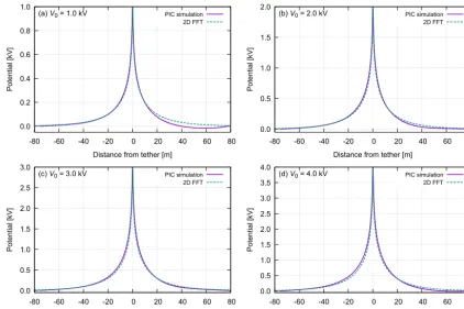
The proposed estimation method was used to obtain a re-alistic potential without performing the full PIC simulation. To realize an equipotential within the radius of the tether, the capacity matrix method was also used (Hockney and East-wood, 1981). Figure 8 compares the potential structures ob-tained using the 2-D FFT method with the PIC results. A cell width ofh=0.03 andN=8192 cells in 2-D space were used for the Fourier transformation. The potential structures estimated using the proposed method were consistent with those obtained from the PIC simulation results (Fig. 5). At

V0=1 kV, there was a small difference (approximately 20 V) between the potential structures estimated using the proposed

method and the PIC simulation results behind the tether, but this difference did not cause a difference in the thrust, be-cause only the potential in front of the tether contributes to the thrust.

3.2 Effective radius method (Method 1)

Method 1 considers the effective radiusrs that satisfies the

following equation:

eV (rs)=

1 2mpv

2

d, (9)

wherers is the distance from the tether at which the

electro-static potential energy is equal to the kinetic energy of the drifting proton. Janhunen and Sandroos (2007) assumed that the scattering cross section is proportional tors with a

0.0 0.2 0.4 0.6 0.8 1.0

-80 -60 -40 -20 0 20 40 60 80

(a) V0 = 1.0 kV

Potential [kV]

Distance from tether [m] PIC simulation

2D FFT

0.0 0.5 1.0 1.5 2.0

-80 -60 -40 -20 0 20 40 60 80

(b) V0 = 2.0 kV

Potential [kV]

Distance from tether [m] PIC simulation

2D FFT

0.0 0.5 1.0 1.5 2.0 2.5 3.0

-80 -60 -40 -20 0 20 40 60 80

(c) V0 = 3.0 kV

Potential [kV]

Distance from tether [m] PIC simulation

2D FFT

0.0 0.5 1.0 1.5 2.0 2.5 3.0 3.5 4.0

-80 -60 -40 -20 0 20 40 60 80

(d) V0 = 4.0 kV

Potential [kV]

Distance from tether [m] PIC simulation

2D FFT

Figure 8.Comparison of potential structures at surface potentials of(a)V0=1 kV,(b)V0=2 kV,(c)V0=3 kV, and(d)V0=4 kV. Blue

lines show the potential structure obtained using the proposed method. Purple lines show the results of the PIC simulations.

length dF /dLcan be expressed as dF

dL =KrsPdyn

=Krsn0mpvd2, (10)

where Pdyn=mpn0vd2 is the dynamic pressure of a solar wind proton.

In Janhunen and Sandroos (2007), V (r) is given by Eq. (1). In the present study,V (r)was replaced with the nu-merical solution obtained using the 2-D FFT method, which considers potential shielding by ambient electrons. For the numerical calculation, the value ofr that minimizes the dif-ference between the potential energy and the kinetic energy

f1, which is expressed as

f1(r)=eV (r)− 1 2mpv

2

d, (11)

is used asrs instead the value ofr. The coefficient of

propor-tionality was set toK=3.09, as obtained by Janhunen and Sandroos (2007).

3.3 Coulomb scattering method (Method 2)

The thrust modeling method by Sanchez-Torres (2014) is based on Coulomb scattering. The following equation is formed by adding an angular momentum term to Eq. (9):

eV (r)+ L

2 m 2mpr2

=1

2mpv 2

d, (12)

whereLm=mpvdρ is the angular momentum and ρ is the impact parameter. DefiningEsw=1₂mpv2_dyields

eV (r) Esw

+ρ

2

r2 =1. (13)

Additionally,landUeffwere defined as

l≡ρ

r (14)

Ueff(l)≡

eV (r) Esw

+l2. (15)

Ueff(l)is equal to the left-hand side of Eq. (13), meaning the distancermin that minimizesf2(ρ_r)=1−Ueff(ρ_r)is equiv-alent to the distance rs obtained using the effective radius

0 20 40 60 80 100 120 140

0.5 1.0 1.5 2.0 2.5 3.0 3.5 4.0

Estimated thrust per unit length [nN

m ] Potential [kV] PIC simulation Janhunen and Sandroos (2007) Sanchez-Torres (2014)

Method 1 (based on Janhunen and Sandroos, 2007) Method 2 (based on Sanchez-Torres, 2014)

Method 1 (effective radius)

Method 2 (Coulomb scattering)

-1

Figure 9.Comparison of thrust estimations. The purple line shows the modified estimation obtained using the effective radius method. The green line shows the modified estimation based on the Coulomb scattering method. The blue and black lines are the same as those in Fig. 4.

δ(ρ)=ρ

   rmax Z r_min dr r2 q

1−ρ2

r2 − eV (r) Esw + ∞ Z rmax dr r2 q

1−ρ2

r2 





(16)

=δ1(ρ)+δ2(ρ) (17)

δ1(ρ)=

lmax Z

lmin

dl √

1−Ueff(l)

(18)

δ2(ρ)=

lmin Z

0 dl √

1−l2=sin(lmin), (19)

where lmax=ρ/rmin and lmin=ρ/rmax. rmax denotes the maximum length that scattered particles can be affected by an electrostatic potential. rmax was defined as rshe−b by Sanchez-Torres (2014) and has been calculated as follows by Sanmartín et al. (2008):

1.53

"

1−2.56

_λ

D

rsh

4/5#_r

sh

λD

4/3

ln

_r

sh

rw

= eV0 kBTe

. (20)

Then, the thrust per unit length can be expressed as

dF

dL =n0vd×2 rmax

Z

0

2mpvdsin χ (ρ) 2 cos

π−χ (ρ) 2

dρ (21)

=4Pdyn

rmax Z 0 sin2 _{χ (ρ)} 2

dρ. (22)

In the present estimation,V (r)in Eq. (15) was replaced with the numerical solution obtained using the 2-D FFT method, and the maximum affection length rmax=2.0λD was used instead of the value of rmax=rshe−b used by Sanchez-Torres (2014).

3.4 Estimation results

The thrust per unit length was obtained forV0=0 to 4.0 kV withrw=15 cm. Figure 9 shows the thrust estimated using

the effective radius method (purple line) and the Coulomb scattering method (green line). These modified thrust esti-mations are similar to the thrust obtained from the PIC simu-lation, meaning they are also significantly lower than estima-tions from previous studies. The modified estimated thrusts obtained using Methods 1 and 2 are 79.1 and 62.0 nN m−1, respectively. The thrust estimated using Method 2 at 4.0 kV is in very good agreement with the PIC result of 67.1 nN m−1. It should be noted that the difference between the modified and previous estimation methods is simply the electrostatic potential structure. The effective proton deflection area with shielding is smaller than that without the shielding. Thus, the inclusion of potential shielding results in reduced thrust.

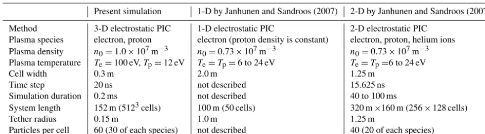
coeffi-Table 2.Differences between the present PIC simulation and those by Janhunen and Sandroos (2007).

Present simulation 1-D by Janhunen and Sandroos (2007) 2-D by Janhunen and Sandroos (2007)

Method 3-D electrostatic PIC 1-D electrostatic PIC 2-D electrostatic PIC

Plasma species electron, proton electron (proton density is constant) electron, proton, helium ions

Plasma density n0=1.0×107m−3 n0=0.73×107m−3 n0=0.73×107m−3

Plasma temperature Te=100 eV,Tp=12 eV Te=Tp=6 to 24 eV Te=Tp=6 to 24 eV

Cell width 0.3 m 2.0 m 1.25 m

Time step 20 ns not described 15.625 ns

Simulation duration 0.2 ms not described 40 to 100 ms

System length 152 m (5123cells) 100 m (50 cells) 320 m×160 m (256×128 cells)

Tether radius 0.15 m 1.0 m 1.25 m

Particles per cell 60 (30 of each species) not described 40 (20 of each species)

cient; thus, the Coulomb scattering method was considered to be more consistent with the PIC results.

4 Discussion

In this study, a full PIC simulation of the E-sail was con-ducted. The most significant difference between the results obtained in this paper and those obtained in previous studies is that the electrostatic potential structure around the tether was considered, which yielded different values of the thrust. In the PIC simulation by Janhunen and Sandroos (2007), the potential shielding effect of the ambient electrons was not significant. In the analytical estimation by Sanchez-Torres (2014), they assumed the absence of ambient electrons so their estimations of the potential (Eq. 3) were higher than those obtained using Eq. (1) at high positive potentials. In the present PIC simulation, the ambient electrons shield the po-tential of the tether more effectively than those in Janhunen and Sandroos (2007) and Sanchez-Torres (2014).

This study focused on the source of the differences be-tween the present PIC simulation and the PIC simulations performed by Janhunen and Sandroos (2007), which are shown in Table 2.

There are several differences among the simulations, par-ticularly regarding the tether dimensions, plasma conditions, simulation duration, and cell width. We consider that the dif-ferences caused the disagreement of the simulation result. Note that the electron temperature kBTe=100 eV adopted in this paper is the typical value in solar wind at 0.5 AU and is about 1 order of magnitude higher than the typical value at 1 AU (applied in previous studies).

To the best of the authors’ knowledge, this study is the first to perform a full 3-D PIC simulation of the E-sail without any approximations. The radius of the tether (rw=15 cm)

was large in comparison with several tens of micrometers; thus, the E-sail was not completely simulated, but the dif-ference is negligible because 15 cm is much smaller thanλD (approximately several meters to a few tens of meters in

in-terplanetary space), so the ambient electron collection is not significantly different.

The increase in thrust caused by the removal of electrons, which was discussed by Janhunen (2009), was not investi-gated in this study; the present simulation did not consider multiple tethers, and the simulation duration (0.2 ms) was not long enough to describe such a effect. If any efficient trapped electron removal mechanisms exist, the thrust of E-sail may increase asymptotically, so we must remark that the thrust characteristics obtained in this paper do not consider the effect of the trapped electron removal. However, the pre-sented simulation successfully described the response of am-bient electrons as shown in Fig. 3. Hence, our results reveal at least the minimum thrust characteristics of the E-sail.

A modified thrust estimation proposed in this paper, which is obtained by replacing the electrostatic potential structures used in the estimations in the previous studies, is a better reference model of the minimum thrust of the E-sail. The proposed estimation method can be easily used to calculate the minimum thrust of E-sail.

5 Conclusions

In this study, the first full 3-D PIC simulation of the tether of the E-sail was performed, and the transient of its thrust was numerically calculated. AtV0≤4.0 kV, the thrust ob-tained by PIC simulation was almost half of the thrust esti-mated in previous studies. This difference is caused by the electrostatic potential structure around the tether. The poten-tial structure in the present simulation differed greatly from the structure used in previous estimations due to the strong potential shielding by ambient electrons.

results. The proposed method can be easily used to calculate the minimum thrust of E-sail.

In future work, we will perform the long-duration simula-tion and investigate an asymptotic thrust characteristics. We also plan the PIC simulation of a much thinner tether using various simulation techniques, such as the fictitious surface method.

6 Data availability

The PIC simulation data (approximately 1TB), which in-clude potential structure, electric field, and density structure, are available upon requests.

The Supplement related to this article is available online at doi:10.5194/angeo-34-845-2016-supplement.

Author contributions. K. Hoshi improved the performance of the PIC code, performed the PIC calculation, analyzed the results, wrote the thrust estimation code, and wrote the paper. H. Kojima and H. Yamakawa directed the study and discussed the interpreta-tion of the results. T. Muranaka first developed the full PIC code and helped run the code on the supercomputer system.

Acknowledgements. The computations in the present study were performed using the Kyoto-daigaku Denpa-kagaku Keisanki-jikken (KDK) system at the Research Institute for Sustainable Hu-manosphere (RISH) at Kyoto University. The present study was supported by JSPS KAKENHI Grant-in-Aid for JSPS Fellows Number 15J08941.

The topical editor, E. Roussos, thanks T. Lafleur and one anony-mous referee for help in evaluating this paper.

References

Hockney, R. W. and Eastwood, J. W.: Computer Simulation Using Particles, McGraw-Hill International Book Co., New York, 1981. Hoshi, K., Kojima, H., and Yamakawa, H.: Numerical Analysis of Potential Structure around Electric Solar Wind Sail Tether, Transactions of JSASS Aerospace Technology, in press, 2016. Janhunen, P.: Electric sail for spacecraft propulsion, J. Propul.

Power, 20, 763–764, 2004.

Janhunen, P.: Increased electric sail thrust through removal of trapped shielding electrons by orbit chaotisation due to space-craft body, Ann. Geophys., 27, 3089–3100, doi:10.5194/angeo-27-3089-2009, 2009.

Janhunen, P. and Sandroos, A.: Simulation study of solar wind push on a charged wire: basis of solar wind electric sail propulsion, Ann. Geophys., 25, 755–767, doi:10.5194/angeo-25-755-2007, 2007.

Muranaka, T., Shinohara, I., Funaki, I., Kajimura, Y., Nakano, M., and Tasaki, R.: Research and development of plasma simulation tools in JEDI/JAXA, Journal of Space Technology and Science, 25, 1–18, 2011.

Sanchez-Torres, A.: Propulsive Force in an Electric Solar Sail, Con-trib. Plasma Phys., 54, 314–319, 2014.