Challenges associated with modeling low-oxygen waters in Chesapeake Bay: a multiple model comparison

www.biogeosciences.net/13/2011/2016/ doi:10.5194/bg-13-2011-2016

© Author(s) 2016. CC Attribution 3.0 License.

Challenges associated with modeling low-oxygen waters

in Chesapeake Bay: a multiple model comparison

Isaac D. Irby1, Marjorie A. M. Friedrichs1, Carl T. Friedrichs1, Aaron J. Bever2, Raleigh R. Hood3, Lyon W. J. Lanerolle4,5, Ming Li6, Lewis Linker7, Malcolm E. Scully8, Kevin Sellner9, Jian Shen1, Jeremy Testa6, Hao Wang3, Ping Wang10, and Meng Xia11

1_{Virginia Institute of Marine Science, College of William & Mary, P.O. Box 1346, Gloucester Point, VA 23062, USA} 2_{Anchor QEA, LLC, 130 Battery Street, Suite 400, San Francisco, CA 94111, USA}

3_{Horn Point Laboratory, University of Maryland Center for Environmental Science, P.O. Box 775, Cambridge,} MD 21613, USA

4_{NOAA/NOS/OCS Coast Survey Development Laboratory, 1315 East–West Highway, Silver Spring, MD 20910, USA} 5_{ERT Inc., 14401 Sweitzer Lane Suite 300, Laurel, MD 20707, USA}

6_{Chesapeake Biological Laboratory, University of Maryland Center for Environmental Science, P.O. Box 38, Solomons,} MD 20688, USA

7_{US Environmental Protection Agency Chesapeake Bay Program Office, 410 Severn Avenue, Annapolis, MD 21403, USA} 8_{Woods Hole Oceanographic Institution, Applied Ocean Physics and Engineering Department, Woods Hole, MA 02543, USA} 9_{Chesapeake Research Consortium, 645 Contees Wharf Road, Edgewater, MD 21037, USA}

10_{VIMS/Chesapeake Bay Program Office, 410 Severn Avenue, Annapolis, MD 21403, USA} 11_{Department of Natural Sciences, University of Maryland Eastern Shore, MD, USA}

Correspondence to: Isaac D. Irby ([email protected]) and Marjorie A. M. Friedrichs ([email protected])

Received: 2 December 2015 – Published in Biogeosciences Discuss.: 21 December 2015 Revised: 8 March 2016 – Accepted: 9 March 2016 – Published: 6 April 2016

Abstract. As three-dimensional (3-D) aquatic ecosystem models are used more frequently for operational water qual-ity forecasts and ecological management decisions, it is im-portant to understand the relative strengths and limitations of existing 3-D models of varying spatial resolution and bio-geochemical complexity. To this end, 2-year simulations of the Chesapeake Bay from eight hydrodynamic-oxygen mod-els have been statistically compared to each other and to his-torical monitoring data. Results show that although models have difficulty resolving the variables typically thought to be the main drivers of dissolved oxygen variability (stratifica-tion, nutrients, and chlorophyll), all eight models have sig-nificant skill in reproducing the mean and seasonal variabil-ity of dissolved oxygen. In addition, models with constant net respiration rates independent of nutrient supply and temper-ature reproduced observed dissolved oxygen concentrations about as well as much more complex, nutrient-dependent biogeochemical models. This finding has significant ramifi-cations for short-term hypoxia forecasts in the Chesapeake

1 Introduction

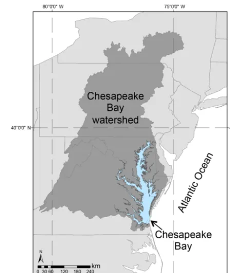
Since the middle of the last century, anthropogenic impacts have dramatically decreased water quality throughout the Chesapeake Bay (Boesch et al., 2001), one of the largest es-tuaries in North America. Land-use change along with the in-dustrialization and urbanization of the Chesapeake Bay wa-tershed have caused dramatic increases in nutrient inputs to the bay (Kemp et al., 2005), spurring additional primary pro-duction and phytoplankton abundance (Harding Jr. and Perry, 1997). Because increased primary production leads to more organic matter throughout the water column that is eventu-ally decomposed by bacteria, these increased nutrient inputs to the bay have led to a corresponding decrease in dissolved oxygen (DO) concentrations (Hagy et al., 2004). Hypoxia, generally defined as the condition in which DO concentra-tions are below 2 mg L−1_{, usually initiates seasonally in the} northern portion of the bay and expands southward as sum-mer develops (Kemp et al., 2009; Testa and Kemp, 2014). Although hypoxia in the Chesapeake Bay has likely ex-isted since European colonization (Cooper and Brush, 1991, 1993), recent studies have highlighted an accelerated rise in the number and spatial extent of hypoxic, as well as anoxic (DO concentrations <0.2 mg L−1), events in the bay since the 1950s, primarily attributed to increased anthropogenic nutrient input (Hagy et al., 2004; Kemp et al., 2005; Gilbert et al., 2010). These impacts are likely to be exacerbated by future climate change (Najjar et al., 2010; Meire et al., 2013; Harding Jr. et al., 2015).

Interest in the ecological impacts of reduced DO con-centrations has been elevated due to the observed prolifer-ation of hypoxic events in the world’s coastal oceans, cre-ating vast dead zone areas that compress suitable habitats for many marine species (Diaz, 2001; Diaz and Rosenberg, 2008; Pierson et al., 2009). Low-DO waters can greatly impact the abundance and health of important ecological species, potentially resulting in suffocation and major kills of fish, crabs, and shellfish (Breitburg, 2002; Ekau et al., 2010; Levin et al., 2009). While the presence of DO concentra-tions <2 mg L−1 have been shown to decrease the abun-dance of fish larvae (Keister et al., 2000), some species can incur negative health impacts and modify their behavior at significantly higher DO concentrations (Vaquer-Sunyer and Duarte, 2008). DO concentrations of∼4 mg L−1have been found to compress demersal fish habitat as fish seek out more oxygenated waters (Buchheister et al., 2013). Zooplankton, a crucial food source for valuable species, have also been found to exhibit changes in distribution and predation when subject to large volumes of low-DO water, potentially lead-ing to further impacts along the food chain (Breitburg et al., 1997; Pierson et al., 2009). Invertebrates have similarly been found to alter their behavior under low-DO condi-tions (Riedel et al., 2014). In the Chesapeake Bay, multi-ple regulated fish species, such as striped bass and American shad, require oxygen restoration targets as high as 5 mg L−1

Figure 1. Map of the Chesapeake Bay and its watershed.

(USEPA, 2010). The greatest impact of low DO concentra-tions spatially will depend on the specific living resource; however, temporally, late spring to early fall is of most con-cern. As a result of the significant ecological importance of oxygen on living resources in the bay, DO concentrations are used as a primary indicator in assessing water quality for Chesapeake Bay regulations (Keisman and Shenk, 2013).

Many 3-D hydrodynamic-oxygen models of varying com-plexity stemming from the academic research community have also been used to simulate DO concentrations through-out the Chesapeake Bay (Scully, 2010, 2013; Hong and Shen, 2013; Feng et al., 2015; Testa et al., 2014; Y. Li et al., 2015). Bever et al. (2013) specifically demonstrated that multiple models of varying complexity are able to generate skillful es-timates of hypoxic volume in the bay. Some of these models are being used in the bay to simulate short-term and/or sea-sonal forecasts of DO conditions. Furthermore, some models are also being used to generate scenario forecasts, or projec-tions, that assess the impact of changes in management prac-tices on estuarine DO concentrations, in some cases taking into account the impacts of future changes in climate.

As ecosystem and water quality models are increasingly used for operational forecasts as well as scenario-based management decisions by the regulatory and academic re-search communities, it is important to understand the rela-tive strengths and limitations of existing models of varying complexity. The ability to discern which variables must be most accurately simulated in order to adequately reproduce the temporal and spatial variability of bay oxygen concentra-tions is a necessary prerequisite for fully understanding how volumes of low-DO water are initiated and sustained within water quality models. The utilization of multiple models can also inform projections by providing independent confidence bounds for management decisions. To those ends, the over-arching goals of this research are to compare the relative skill of various 3-D Chesapeake Bay models characterized by different levels of biogeochemical complexity and spatial resolution, to better understand factors limiting their ability to reproduce observed DO distributions, and to suggest ap-proaches for the continued improvement of these models.

2 Methods

2.1 Participating Chesapeake Bay models

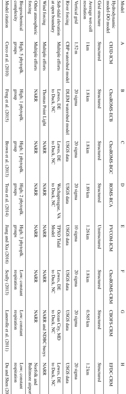
Eight 3-D models were evaluated in this study (Table 1), each of which includes hydrodynamic and DO components. Among the eight models, there are four different hydrody-namic base models. Models B, C, D, F, and G utilize the Regional Ocean Modeling System (ROMS; Shchepetkin and McWilliams, 2005; Haidvogel et al., 2008) that employs a structured grid with sigma layers in the vertical dimension. Specifically, Models B, C, and F use a ROMS implemen-tation developed for the Chesapeake Bay based on Xu et al. (2012; ChesROMS). Model D employs a ROMS im-plementation for the Chesapeake Bay based on M. Li et al. (2005), while Model G uses the ROMS-based Chesapeake Bay Operational Forecast System (CBOFS; Lanerolle et al., 2011). Models A, E, and H each use a different hydrody-namic base model: the Curvilinear Hydrodyhydrody-namics in Three Dimensions model (CH3D; Cerco et al., 2010), the

Finite-Volume Community Ocean Model (FVCOM; Jiang and Xia, 2016), and the Hydrodynamic Eutrophication Model – Envi-ronmental Fluid Dynamics Code (EFDC; Park et al., 1995; Hong and Shen, 2012; Du and Shen, 2015), respectively. The only model that employs a non-sigma vertical grid is Model A and the only model utilizing an unstructured hor-izontal grid is Model E. While Model E contains 10 sigma vertical layers, all of the other sigma grids use 20 layers. All of the grids vary in terms of their horizontal resolution, with Models A and G utilizing the highest resolution horizontal grids.

These four hydrodynamic models are coupled to five dif-ferent models used to simulate DO (Table 1). Models A, B, C, D, and E utilize full biogeochemical models that include various combinations of oxygen, phytoplankton, zooplank-ton, and multiple inorganic and organic nutrients as state variables. Specifically, Models A and E employ a version of the Integrated Compartment Model (ICM; Cerco et al., 2010; Jiang et al., 2015), Model B uses the Estuarine Carbon Bio-geochemistry model (ECB; Feng et al., 2015), Model C uses the Biogeochemistry model (BGC; Brown et al., 2013), and Model D uses the Row–Column AESOP model (RCA; Testa et al., 2014). In terms of food web complexity the models vary considerably: Models B and C employ a single phyto-plankton group whereas Model D uses two phytophyto-plankton groups, Model E uses three, and Model A, the most complex of the participating models, uses five.

In contrast to the full biogeochemical models discussed above (Models A through E), Models F, G, and H represent oxygen dynamics as simply as possible and therefore do not utilize a full biogeochemical component. Rather, the models impose a biological oxygen consumption rate that is model-specific, but constant in both space and time. This compo-nent is referred to as a constant-respiration model (CRM). In this model, DO is introduced to the estuary via the river and ocean boundaries and is set to saturation at the estuar-ine surface. This constant-respiration oxygen parameteriza-tion (Scully, 2010) is simplistic, yet has been shown to ade-quately represent Chesapeake Bay oxygen dynamics (Scully, 2010, 2013; Bever et al., 2013).

Mod-T able 1. Model characteristics. Model A B C D E F G H Hydrodynamic CH3D-ICM ChesR OMS-ECB ChesR OMS-BGC R OMS-RCA FVCOM-ICM ChesR OMS-CRM CBOFS -CRM EFDC-CRM model-DO model Grid structure Structured Structured Structured Structured Unstructured St ructured Structured Structured A v erage wet-cell 1 km 1.8 km 1.8 km 1.89 km 1.26 km 1.8 km 0.565 km 1.2 km resolution V ertical grid 1.52 m 20 sigma 20 sigma 20 sigma 10 sigma 20 sigma 20 sigma 20 sigma Ri v er forcing CBP w atershed model DLEM w atershed model USGS data USGS data USGS data USG S data USGS data USGS data Sub-tidal ele v ation Multiple ef forts Le wes, DE Le wes, DE W achapreague, V A TPXO T idal Le w es, DE Ocean City , MD Le wes, DE at open boundary to Duck, NC to Duck, NC to Duck, NC Model to Duck, NC to Duck, NC to Duck, NC W ind forcing Multiple ef forts Thomas Point Light N ARR N ARR N ARR N ARR N ARR and NDBC b uo ys N ARR Other atmospheric Multiple ef forts N ARR N ARR N ARR N ARR N ARR N ARR Norfolk and forcing Baltimore airports Biogeochemical High; 5 ph ytoplk. High; 1 ph ytoplk. High; 1 ph ytoplk. High; 2 ph ytoplk. High; 3 ph ytoplk. Lo w; cons tant Lo w; constant Lo w; constant comple xity groups group group groups groups respiration respiration respiration Model citation Cerco et al. (2010) Feng et al. (2015) Bro wn et al. (2013) T esta et al. (2014) Jiang and Xia (2016) Scull y (2013) Lanerolle et al. (2011) Du and Shen (2015)

els C through H use wind estimates from the North American Regional Reanalysis (NARR).

The eight models used in this analysis have been devel-oped for a variety of purposes. Model A is a governmental regulatory model developed by the CBP that has been exten-sively calibrated specifically to examine water quality issues in the Chesapeake Bay (Cerco and Cole, 1993; Cerco and Noel, 2004, 2013; Cerco et al., 2010) and has been used in the development of the 2010 Chesapeake Bay Total Maximum Daily Load (USEPA, 2010). The National Oceanic and At-mospheric Administration employs the hydrodynamic com-ponent of Model F for operational forecasts of a variety of physical estuarine parameters for the Chesapeake Bay (http: //www.tidesandcurrents.noaa.gov/ofs/cbofs/cbofs.html). The other six models are academic models used in diverse re-search efforts focused on the Chesapeake Bay but not nec-essarily specifically on DO dynamics.

Finally, a ninth model is calculated as the mean of the re-sults from the eight models described above, and is referred to here as Model Mean, or Model M.

2.2 Available Chesapeake Bay observations

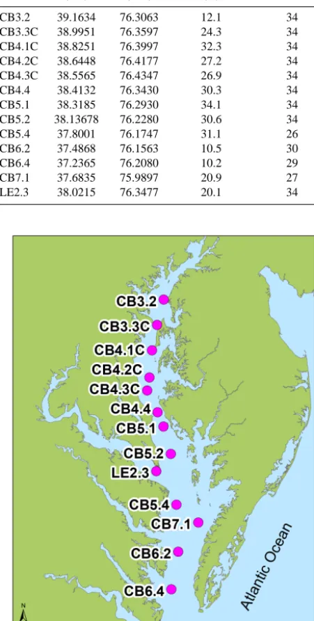
Table 2. Characteristics of observation stations (from USEPA,

2012).

Station Latitude Longitude Station depth No. of cruises (◦N) (◦W) (m)

CB3.2 39.1634 76.3063 12.1 34 CB3.3C 38.9951 76.3597 24.3 34 CB4.1C 38.8251 76.3997 32.3 34 CB4.2C 38.6448 76.4177 27.2 34 CB4.3C 38.5565 76.4347 26.9 34 CB4.4 38.4132 76.3430 30.3 34 CB5.1 38.3185 76.2930 34.1 34 CB5.2 38.13678 76.2280 30.6 34 CB5.4 37.8001 76.1747 31.1 26 CB6.2 37.4868 76.1563 10.5 30 CB6.4 37.2365 76.2080 10.2 29 CB7.1 37.6835 75.9897 20.9 27 LE2.3 38.0215 76.3477 20.1 34

Figure 2. Location of the CBP water quality monitoring stations

used in this study.

2.3 Calculation of stratification and mixed layer depth Stratification of the density and oxygen fields was examined to identify the maximum gradient of the pycnocline and oxy-cline as well as the depth of the top of the pycnooxy-cline and oxycline. In open ocean studies, the depth of the top of strat-ification is commonly referred to as the mixed layer depth (MLD), although this term is less frequently used in the

estu-arine literature. As the research presented here distinguishes between the depths of the top of the pycnocline and that of the oxycline, these will be referred to respectively as the den-sity (ρ) mixed layer depth (MLDρ) and the oxygen mixed layer depth (MLDO). Density was calculated via a classical density formula that is also utilized by the CBP for use in the Chesapeake Bay (Fofonoff and Millard, 1983; USEPA, 2004) and is a function of temperature and salinity.

The CBP defines the top and bottom of stratification in order to distinguish individual designated use areas for wa-ter quality management purposes (USEPA, 2004). They sug-gest that the top of the pycnocline be defined as the shallow-est occurrence of a density gradient of 0.1 kg m−4or greater as resolved by CBP profile observations, which are typi-cally spaced at 0.5–2 m depth intervals. If density gradients throughout the water column are less than 0.1 kg m−4_{, they} define the water to be unstratified. The 0.1 kg m−4_threshold definition is designed to identify any initiation of stratifica-tion that may serve to cut off vertical mixing from a nearly perfectly well-mixed layer.

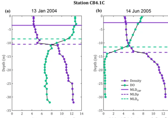
While the CBP definition described above delineates be-tween designated use boundaries according to density, our research focuses on the relationship between the pycnocline and oxycline, requiring an alternate definition that can be applied to both the density and oxygen distributions. In ad-dition, the CBP definition often generates estimates for the depth of the top of the pycnocline that are too shallow com-pared to the maximum depth of surface mixing (Fig. 3). As a result, a percentage threshold criterion was developed that identifies the bottom of the reasonably well-mixed layer, rather than perfectly mixed layer, and is used in this analy-sis. The percentage threshold method defines a density or DO profile as being stratified if a change of 10 % of the difference between the profile’s maximum and minimum values occurs within a single meter (Fig. 3). For example, if the maximum DO concentration throughout the water column on an indi-vidual sampling date is 10 mg L−1 and the minimum con-centration is 1 mg L−1, stratification is defined to be present if a difference of 0.9 mg L−1 is present within 1 m. As rec-ommended by the CBP, the uppermost meter of the water column is not considered (USEPA, 2004). The mixed layer depth is therefore defined as the shallowest level (below 1 m depth) where stratification is identified. The minimum strati-fication criterion utilized in this analysis requiring a profile to pass the 10 % threshold also ensures that observations where very little stratification exists do not bias the stratification results while also allowing for a single criterion to be used across multiple stratification variables.

2.4 Model skill metrics

Figure 3. Density and dissolved oxygen profiles for a mid-bay station (CB4.1C) on (a) 13 January 2004 and (b) 14 June 2005, comparing

the 0.1 kg m−4stratification definition used by the CBP (MLDCBP) with the 10 % threshold definitions used here for density (MLDρ) and oxygen (MLDO).

deviation, and correlation coefficient. These metrics are il-lustrated on Taylor and target diagrams (Taylor, 2001; Hof-mann et al., 2008; Jolliff et al., 2009), which offer a com-pact way of assessing model skill by displaying a number of different skill metrics. Target diagrams illustrate the bias and total RMSD of model output, which Taylor diagrams do not. Taylor diagrams include quantitative information on the standard deviations and correlations between the model output and the observations, which target diagrams do not. Both diagrams, however, represent unbiased RMSD, some-times called “centered-pattern RMSD”. On target diagrams, a model symbol above the horizontal axis overestimates the mean of the observations and a model symbol to the right of the vertical axis overestimates the variability of the obser-vations. (See Hofmann et al. (2008) and Jolliff et al. (2009) for a more detailed description of these diagrams.) On Tay-lor diagrams, a model symbol lying on the horizontal axis exactly correlates to the observations and a model symbol further from the origin than the observation symbol overes-timates the standard deviation of the observations. (See Tay-lor (2001) for a more detailed description of these diagrams.) Taylor and target diagrams presented here are normalized to the standard deviation of the observations, allowing multi-ple variables be represented on the same plot. This also con-veniently allows the unit circle on a target diagram to repre-sent the skill of a model defined as the mean of the obser-vations. In effect, this means that if a model falls within the unit circle, it exhibits a skill that is greater than the skill ob-tained if one were to simply use the mean of the observations. The Taylor and target plots are either temporal (displaying model skill at a single station over the study period) or spa-tial (displaying model skill during a single month over the

en-tire set of study stations). In addition, summary diagrams are presented which combine both temporal (examining the sea-sonal changes at each individual station) and spatial (exam-ining differences across the bay during an individual month) variability.

3 Results

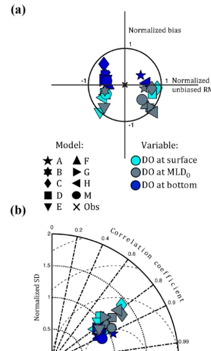
An analysis of model skill of the combined temporal and spatial variability of DO at the surface and bottom of the water column, as well as at the observed MLDO, indicates that all models, regardless of biogeochemical complexity or spatial resolution, exhibit a high degree of skill in reproduc-ing observed DO (Fig. 4). Specifically, all models produce DO concentrations at the surface and bottom that have a nor-malized total RMSD less than 1. The same is true for nearly all models for DO at the observed MLDO. However, most models underestimate observed DO both at the surface and at the MLDO(Fig. 4a). The correlation between the observed and modeled DO is relatively constant with depth (Fig. 4b), though on average slightly higher at the bottom (0.85) than at the surface (0.80). Further, on average, the models sim-ulate DO at the surface and bottom better than they do at the MLDO. No statistical difference exists between the skill of models that utilize a full biogeochemical component and those that utilize the simple constant-respiration oxygen pa-rameterization. Based on an analysis of variance (ANOVA) comparing the full biogeochemical models to the CRM mod-els, the two model types do not perform differently in terms of their ability to reproduce the combined temporal and spa-tial variability of bottom DO as measured by total RMSD (p=0.48). Overall, Model M (the mean of the eight mod-els) consistently performs better than any individual model across all depths examined (Fig. 4).

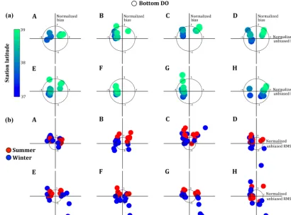
The monthly temporal variability of bottom DO at each station over the 2 years studied is resolved similarly well by all of the models (Fig. 5a), but the models have difficulty sim-ulating spatial DO variability during each month (Fig. 5b). Due to the stations chosen for this analysis (Fig. 2), the spa-tial variability being examined here is essenspa-tially the north to south variability. Most models exhibit a latitudinal gra-dient with respect to their skill in reproducing the temporal variability of bottom DO, with models overestimating DO at the more northern stations (Fig. 5a). Some models dif-fer in their ability to reproduce summer (May–September) DO concentrations and winter (October–April) DO concen-trations (Fig. 5b). Models B, F, and G all distinctively over-estimate mean DO in the summer compared to the winter. In contrast, Models A and C perform similarly well in both seasons (Fig. 5b). In addition, all three constant respiration models, as well as Models D and E, substantially underesti-mate DO at several stations in the winter.

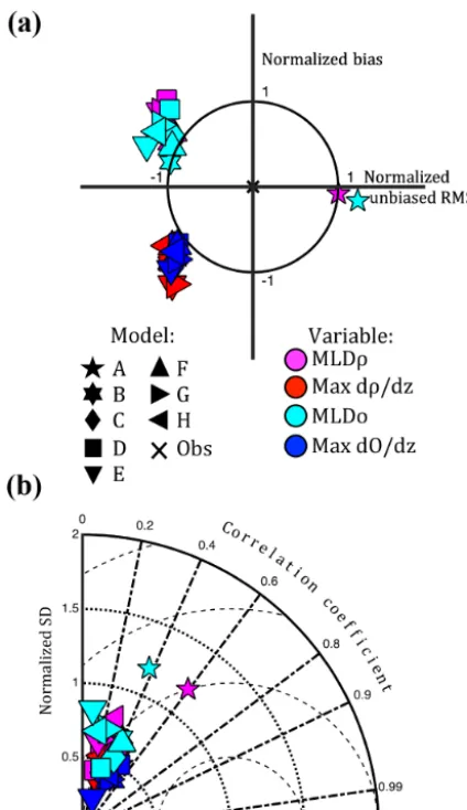
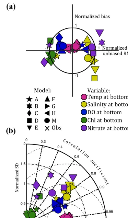
All eight models generally resolve the pycnocline and oxy-cline with similar skill (Fig. 6). All models consistently un-derestimate the mean and standard deviation of the maximum strength of stratification within the pycnocline and oxycline, defined herein as the maximum vertical gradients of density and oxygen (Fig. 6a). All models, except for Model A (see Sect. 4.2), also underestimate the mixed layer depth, regard-less of whether it is computed in terms of density or oxy-gen. (Note that these model symbols in Fig. 6a are located

Figure 4. Normalized summary (a) target and (b) Taylor diagrams

illustrating model skill of dissolved oxygen at the surface, MLDO, and bottom for 13 Chesapeake Bay stations in 2004–2005. The “x” represents the skill of a model that perfectly reproduces the obser-vations. The dotted, dashed-dot, and dashed lines on the Taylor dia-gram represent lines of constant standard deviation, correlation co-efficient, and unbiased RMSD, respectively.

above they axis despite this negative bias in MLD because the vertical coordinate system is oriented upwards.) Thus, the models are producing stratification that is both weaker than observed and higher (shallower) in the water column. The correlation coefficient for these metrics is low, ranging 0.1– 0.6, and indicates that all models are missing the majority of variability associated with the magnitude and location of the pycnocline and oxycline (Fig. 6b). However, there is slightly more consistency and better correlation coefficients among the models for the strength of stratification than the depth of the mixed layers.

Figure 5. Normalized target diagrams for Models A–H demonstrating the (a) temporal and (b) spatial skill in resolving the variability of

bottom dissolved oxygen concentrations. In (a) the individual dots represent the 13 stations along the main stem of the Chesapeake Bay. In (b) the dots represent the 24 months of 2004–2005 and are delineated by color: red is summer (May–September) and blue is winter (October–April).

the pycnocline and MLDρ, with model skill generally lower at the northern stations (Fig. 7a). Contrary to the pattern shown for bottom DO (Fig. 5b), none of the models exhibit a significant seasonal pattern between summer and winter in reproducing spatial variability of dρ/dzor MLDρ(Fig. 7b). However, Model A differentiates itself from the rest of the models in its pattern of skill at reproducing the spatial and temporal variability of the MLDρ (see Sect. 4.2). Tempo-ral and spatial patterns for oxycline stratification (dO/dz) and MLDO closely match those of dρ/dzand MLDρ (not shown).

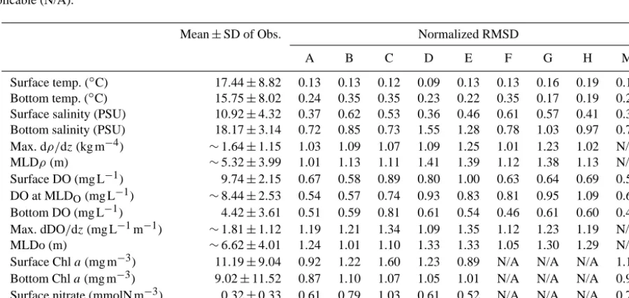
All eight models reproduce the variability of bottom DO better than the variables that are generally thought of as being the primary drivers of hypoxic conditions, including stratifi-cation (Fig. 6), salinity, chlorophyll, and nitrate (Fig. 8, Ta-ble 3). However, all models reproduce patterns in tempera-ture across the bay and through time better than any of the other variables in this model comparison (Fig. 8). All eight models, as well as the Model Mean, are characterized by very low bias in modeled temperature, and correlation coeffi-cients of approximately 0.99; this high skill results from the very strong and predictable seasonal temperature variability.

Even though the five models with full biogeochemical com-ponents (Models A, B, C, D, E) are characterized by large differences in their mechanistic approaches to modeling ni-trate and chlorophyll, they produce similar total RMSDs for all of the variables examined at both the surface and the bot-tom (Table 3).

Figure 6. Normalized summary (a) target and (b) Taylor diagram

illustrating model skill of MLDρand MLDO, max dρ/dz, and max dO/dzat 13 Chesapeake Bay stations for 2004–2005. The “x” rep-resents the skill of a model that perfectly reproduces the observa-tions. Since RMSD of stratification is only computed at stations where both the observations and model exhibit stratification, the Model Mean is not calculable for these variables.

a premature relaxing of hypoxic conditions for both years at this observation station.

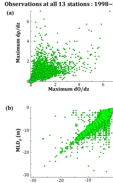
In order to better understand the impact of stratification on DO concentrations throughout the water column, the re-lationship between the observed pycnocline strength and MLDρwere compared to the observed oxycline strength and MLDO. Observations from 1998 to 2006 demonstrate that while there is not a strong correlation between the strengths of the pycnocline and oxycline, there is a very strong corre-lation between MLDρ and MLDO (Fig. 10). Depending on the criteria used for defining the existence of stratification (see Sect. 2.3), the correlation of the pycnocline and oxy-cline strengths ranger2=0.18–0.26 and the correlations of MLDρand MLDO ranger2=0.51–0.82 (Table 4). Further-more, correlation of the relationship between the MLDρand

MLDO is stronger for more severe stratification (Table 4). The relationship between the two mixed layer depths is bi-ased towards the MLDObeing located slightly deeper in the water column than the MLDρ. As the cut-off criteria for the existence of stratification becomes more stringent, the rela-tionship becomes closer to 1:1.

4 Discussion

4.1 How does the skill of various hydrodynamically based DO models compare?

In examining the eight 3-D models in this study, there is not a statistical difference between the abil-ity of simple and complex models to simulate the mean and monthly variability of bottom DO; in ad-dition, models with higher spatial resolution do not necessarily produce better estimates of DO.

Models currently simulating hypoxia throughout Chesa-peake Bay compute oxygen concentrations in essentially two distinct ways: they either utilize a simple constant respiration model or a full biogeochemical model. In this study, the rel-ative skill of both types of models is compared. Specifically, in examining results of the comparison between five biogeo-chemical models (A, B, C, D, E) and three simplistic constant respiration models (F, G, H), the two groups of models per-formed statistically similar in their skill of reproducing bot-tom DO concentrations (Fig. 3, Table 3). These results sup-port those of Bever et al. (2013) who compared three constant respiration models with the CBP regulatory model (Model A) and similarly found that all four of the models were equally skillful in terms of reproducing the seasonal variability in bottom DO throughout the bay in 2004 and 2005. Consis-tent with the results of Scully (2013), this result implies that the seasonal variability of DO in the Chesapeake Bay is pri-marily dependent on underlying hydrodynamic mechanisms which are nearly identical for all eight models, rather than on aspects related to the biogeochemical cycling which vary dramatically between models and in fact are constant in three of the eight models. It should be noted, however, that the 2 years studied here were relatively wet years and an analysis of dry years may offer different results.

neces-Figure 7. Normalized target diagrams for Models A–H demonstrating the (a) temporal and (b) spatial skill in resolving the variability of

the strength of density stratification (circles) and the depth of pycnocline initiation (diamonds). In (a) the individual dots represent the 13 stations along the main stem of the Chesapeake Bay. In (b) the dots represent the 24 months of 2004–2005 and are delineated by color: red is summer (May–September) and blue is winter (October–April).

Table 3. Mean and standard deviation (SD) of observations and total normalized RMSD for each model. RMSD for each model except when

not applicable (N/A).

Mean±SD of Obs. Normalized RMSD

A B C D E F G H M

Table 4. Pycnocline and oxycline correlation statistics (all

correla-tions havepvalues0.01).

Stratification Max. dρ/dz MLDρ Profiles

threshold vs. vs. with

percentage ( %) max. dO/dz MLDO stratification

10 0.18 0.51 1613

15 0.22 0.59 1303

20 0.22 0.70 916

25 0.26 0.82 575

sarily improve model–data agreement. In this case, the in-crease in model complexity has likely outpaced the ability of the researchers to fully tune the model to the available observations. However, even past studies that have invoked formal parameter optimization methodologies, such as ge-netic algorithms and variational adjoint methods (Friedrichs et al., 2007; Ward et al., 2010; Xiao and Friedrichs, 2014), have found that under certain conditions, adding too much complexity does not necessarily improve model skill and in fact can decrease model skill and portability, primarily due to artifacts resulting from overtuning. This mirrors findings from the larger ecosystem modeling community where the best-fit models are often those with intermediate complexity (Fulton et al., 2003).

In this study, horizontal grid resolution differed signifi-cantly between model implementations, with the most highly resolved grid (Model G) including more than 9 times more grid cells than the lower resolution grids (Table 1). A certain degree of resolution is clearly required to successfully sim-ulate dynamic processes, and a model with 8–10 km resolu-tion will not be able to correctly simulate the hydrodynamic processes within the bay (Feng et al., 2015). However, an in-crease in horizontal grid resolution from∼1.8 to∼0.6 km, which results in a run-time change of a factor of 9, or pos-sibly of 27 if the time step is accordingly decreased by a factor of 3, does not necessarily result in a significant im-provement in simulation skill of either stratification or bot-tom oxygen. Although not shown here, additional sensitivity experiments with Model G revealed that doubling the verti-cal resolution of this model had no significant effect on the model’s ability to resolve the depth of stratification or the maximum magnitude of stratification. Thus, when selecting the optimal model resolution for a simulation, it is critical to weigh the advantages of increased resolution with the in-creased time required for simulation. With a given level of computational resources, fewer sensitivity experiments can be conducted with a model using a more highly resolved grid. Accurately simulating the observed spatial variability of DO (Fig. 4b) was a greater challenge than simulating the temporal variability of DO (Fig. 4a) for all eight models par-ticipating in this intercomparison. This is especially true in the winter months when the vast majority of the bay is

oxy-Figure 8. Normalized summary (a) target and (b) Taylor diagram

illustrating model skill of bottom temperature, salinity, chlorophyll, nitrate, and dissolved oxygen at 13 Chesapeake Bay stations for 2004–2005. The “x” represents the skill of a model that perfectly reproduces the observations.

gen replete and the models have difficulty representing the observed variability from station to station. The majority of the models tend to slightly overestimate mean bottom DO in the summer whereas multiple models (e.g., Models D, E, F, and G) exhibit a strong negative bias during January and/or February of 2005, primarily at stations in the middle to south-ern portion of the bay’s deep channel. Interestingly, increased biological complexity and higher grid resolution do not com-pletely resolve this issue, as this is true for models utilizing full biogeochemical models (Models D, E) as well as those using highly resolved model grids (Model G). This is likely due to the ephemeral nature of the biological divers of DO.

Figure 9. Time series of bottom dissolved concentrations for station

CB4.1C. Red dots represent the 34 observations made during 2004– 2005. Grey lines are the individual model simulations. The dark blue line represents the Model Mean while the cyan line represents the 95 % confidence interval of the model simulations.

mixing and temperature) play a dominant role in controlling the seasonal cycle of oxygen (Scully, 2013). Because the un-derlying hydrodynamic models all use similar physical forc-ing, the constant respiration models are able to simulate the seasonal cycle of DO with similar skill as the more com-plex biogeochemical models. As a result, these simple mod-els that are easier to tune and require less in the way of com-putational resources than full biogeochemical models, may be efficiently used to produce short-term (on the order of days) DO forecasts. On the contrary, the more complex full biogeochemical models will be necessary for scenario-based and long-term (on the order of months to years) forecasting which requires that models respond to prescribed changes in the biogeochemical environment, such as increased rates of nutrient loading due to changes in land use, land cover, and/or climate.

4.2 How does model skill of DO compare to that of the primary drivers of DO variability?

Overall, model DO skill is greater than that of the variables generally considered to drive DO vari-ability, such as stratification, salinity, mixed layer depth, chlorophyll, and nitrate; only modeled tem-perature has higher skill than modeled DO.

Since dissolved oxygen concentrations in the Chesapeake Bay are controlled by physical processes (e.g., advection, wind mixing, heating/cooling, and stratification), as well as biological processes (e.g., photosynthesis and respiration), it is critical to understand the skill of the models in terms of how well they reproduce the many factors influencing oxy-gen concentrations. As expected, the five models containing a specific biogeochemical model component had more diffi-culty simulating the observed chlorophyll and nitrate

concen-Figure 10. Scatter plots comparing observations of (a) the strengths

of stratification of the pycnocline and oxycline and (b) the oxygen-and density-defined mixed layer depths. Size of the circles is pro-portional to the number of observations. Observations are from 1998 to 2006 at the 13 Chesapeake Bay stations shown in Fig. 2.

more by physical than biological factors. This also explains the success of the constant respiration models, which by def-inition contain no biological variability yet reproduce DO variability nearly as well as the most complex biogeochemi-cal models.

In this study, model skill was also considerably higher for bottom oxygen than it was for the vertical gradient of strat-ification and mixed layer depths (Figs. 6, 8). The underes-timation of the vertical gradient across all models is largely due to the numerical diffusion that characterizes all of these hydrodynamic models, but may also be partially due to an underestimation of the winds or a lack of diffuse freshwa-ter input around the bay. Even though the models all under-estimated the strength of stratification (Figs. 4, 6), modeled stratification in summer was strong enough to prevent mixing with the relatively well-oxygenated surface waters. This re-sult suggests, somewhat surprisingly, that simulating the cor-rect vertical gradient of stratification is not absolutely neces-sary for skillful bottom DO simulations. Models need only simulate enough stratification to effectively cut off vertical mixing in order to develop an isolated bottom layer that can then experience a draw down in oxygen via respiration. In ad-dition, the models must also correctly simulate the horizontal advection of oxygen (Scully, 2013; Y. Li et al., 2015). The fact that bottom DO is simulated so well by the eight models analyzed here suggests that not only is the advection of oxy-gen well represented in the models but also the strength of stratification, i.e., the maximum vertical gradients of density and oxygen, produced by these models is sufficient. Thus, although novel and somewhat unexpected, these results are not contradictory to previous studies demonstrating the im-portance stratification plays in initiating summer hypoxia in the Chesapeake Bay (Murphy et al., 2011).

Model skill in terms of reproducing observed mixed layer depths was likewise much lower than model skill of repro-ducing observed oxygen concentrations. All models, except Model A, produced mixed layer depths (MLDOand MLDρ) that were generally too shallow in the water column (Fig. 6a). Note that Model A is a regulatory model that has been used for many years by the Chesapeake Bay Program, and has thus undergone more extensive calibration aimed at matching the mean salinity and oxygen characteristics of the bay (Cerco and Cole, 1993). Furthermore, Model A employs a z grid that matches the bathymetry in trench areas better than the sigma grids used by the other models. Although Model A produced mixed layer depths that were generally in the cor-rect location within the water column (Fig. 6a), they were too variable (Fig. 6b). This variability may partly be a result of the 1.5 mzgrid employed by Model A causing large jumps between vertical grid cells and hence resulting in overesti-mates of MLD variability. All other models use sigma grids typically with more highly resolved vertical resolution at the depth of maximum stratification.

The two variables for which the models have greatest skill are DO and temperature (Fig. 8). This is because oxygen

Figure 11. Time series of observations at station CB4.1C from 2003

to 2006 for (a) bottom dissolved oxygen, (b) dissolved oxygen at the MLD_O, and (c) MLD_O.

variability is driven primarily by seasonal variability in phys-ical processes such as solubility and wind mixing and to a lesser degree by variability in oxygen consumption (Scully, 2013). As a result, the models using a constant mean respira-tion rate produce as realistic hypoxia simularespira-tions as the bio-geochemically complex models. Observations clearly show this strong seasonal variability in bottom DO (Fig. 11a) and, to a slightly lesser extent, clear seasonal variability in DO at the bottom of the bottom of the oxygen mixed layer (MLDO; Fig. 11b). However, a seasonal cycle is not manifested in the MLDO itself (Fig. 11c). The lack of such a strong seasonal cycle in the observed mixed layer depths makes this a more difficult variable for the models to simulate. As a result, the models can relatively skillfully simulate the combined spatial and temporal variability of DO while simultaneously missing the MLDO.

4.3 Why is it important for DO models to simulate the MLDOcorrectly?

Most of the aerobic habitat in the bay during the summer is located above the MLDO, thus it is crit-ical for living resource managers to use models that accurately simulate this variable.

Figure 12. Time series of observations of dissolved oxygen and

MLDOcontours at Station CB4.1C for 2004 and 2005.

The severe depletion of oxygen below the mixed layer com-presses the habitable space at this station to roughly 10 m (from a maximum of 32 m) during the annual low-oxygen event.

The impact of habitat compression can be substantial, as many bay species require DO concentrations well above the traditional hypoxic threshold (USEPA, 2010). While not all of the main stem stations develop hypoxic water each year, most mesohaline stations experience a dramatic drawdown of oxygen to levels during the summer that effectively remove a large portion of the bay from habitable space (Murphy et al., 2011; Schlenger et al., 2013). Studies have shown that some species modify their behavior based on the oxycline depth, which acts to constrict the habitable space in the wa-ter column (Prince and Goodyear, 2006; Pierson et al., 2009; Elliott et al., 2013). Since species can be negatively impacted by low-DO concentrations as high as 5 mg L−1_(Breitburg, 2002; Vaquer-Sunyer and Duarte, 2008; USEPA, 2010), the location of the oxycline is not only important for habitat com-pression in the summer months but can also be important in the winter months when an occasional lack of vertical mixing can substantially decrease bottom DO concentrations. Fur-thermore, in order to accurately estimate hypoxic volume, models must correctly simulate the depth of the mixed layer, since the MLDO closely follows the depth of the 2 mg L−1 contour.

4.4 How can DO simulations in the bay be improved for management of water quality and living resources?

To better simulate DO conditions and summer habitat compression due to low-DO water, simu-lations of the depth of the top of the pycnocline (MLDρ) must be improved.

Although the suite of models examined reproduce DO concentrations relatively well overall (Fig. 4), the models typically overestimate summer habitat compression by pro-ducing low DO concentrations too high in the water column (Fig. 6). Observations from the Chesapeake Bay Program show a strong correlation between the depths of the oxy-gen and density-defined mixed layers (Fig. 10b). The mod-els analyzed here also clearly exhibit a close relationship be-tween their skill in simulating the depths of the oxygen and density-defined mixed layers (Fig. 6). These strong relation-ships between the depths of the oxygen and density-defined mixed layers result from the fact that the pycnocline repre-sents the physical barrier that leads to the development of the oxycline. Therefore, the inability of the models to accu-rately simulate habitat compression is an artifact of their lack of skill in simulating the depth of the density-defined mixed layer. In contrast, the strength of density stratification is not well correlated to the strength of oxygen stratification. This is because a relative wide range of intensities of density strat-ification is still sufficient to cut off vertical mixing, leading to the observed draw-down in bottom DO. Thus, even though all models underestimate the strength of the pycnocline, they still produce enough stratification to greatly reduce mixing. The results from this paper thus indicate that to further im-prove DO simulations and better estimate summertime habi-tat compression, it is even more critical for models to accu-rately simulate the depth of the top of the pycnocline than to accurately simulate the absolute strength of the pycnocline. 4.5 What is the utility of the multi-model ensemble and

Model Mean?

The multi-model ensemble approach allows for the development of a model mean, which taken as its own model, is the most skilled model when exam-ining the combined suite of variables analyzed in this study.

placed on models used in regulatory actions, utilization of a multi-model ensemble may not be realistic for all envi-ronmental and resource managers; however, multiple mod-els can be integrated into the decision-making process even when the ultimate decision must be based on a single model. For example, a confidence interval plot could help identify where regulatory model output might be acting out of sync with other skilled water quality models of the same system, thereby informing managers of the potential shortfalls asso-ciated with the regulatory model. Furthermore, if the models tend to be predicting similar DO concentrations, a cohort of models could enhance the confidence in regulatory decisions based on a single regulatory model (Friedrichs et al., 2012; Weller et al., 2013). Comparing multiple models can also help inform how to better improve models in the future, as this study has aimed to do.

5 Conclusions

All models analyzed here exhibited a high degree of skill in simulating dissolved oxygen concentrations within the main stem of the Chesapeake Bay in 2 years corresponding to rel-atively wet and average years. Their high skill results from the fact that physical processes (e.g., solubility, wind-mixing, and advection) exert a first order influence on the seasonal cycle of oxygen. As a result, the models’ ability to reproduce dissolved oxygen concentrations is independent of the com-plexity of the biogeochemical parameterizations: the sim-plest constant respiration models were found to reproduce observed oxygen concentrations as well as the most biologi-cally complex models. Essentially, all models are equally ca-pable of respiring most of the available oxygen in the lower water column during summer.

This study also suggests that for use as management tools for water quality and living resources, it is more critical for these models to adequately resolve the depth of the mixed layer than the absolute strength of stratification (as long as modeled stratification is strong enough to limit vertical mix-ing). This is critical because observations show that during warmer months, oxygen-depleted water fills the water col-umn to where stratification limits further mixing, which ef-fectively cuts off waters below the mixed layer for use by the majority of the Chesapeake Bay’s most recognized and val-ued living resources. These results furthermore suggest that modelers should focus their efforts on improving the hydro-dynamics of their models in an effort to improve simulations of mixed layer depth dynamics and variability.

These findings have significant ramifications for short-term bottom DO forecasts, which may be successful with very simple oxygen parameterizations embedded in hydrody-namic models. In contrast, scenario-based water quality fore-casts are likely to benefit from more complex models, which must adequately reproduce the longer-term response of the oxygen field to changes in nutrient and organic matter loads.

This study also helps to demonstrate how multiple commu-nity models from governmental agencies and academic insti-tutions may be used together to provide a model mean and a set of confidence bounds for regulatory model results that could be used to inform management decisions.

Data Availability

Observations used in this analysis can be downloaded from the Chesapeake Bay Program’s Water Quality Database website at (http://www.chesapeakebay.net/data/downloads/ cbpwaterqualitydatabase1984present). Model output for the individual stations examined in this analysis can be ob-tained by contacting Marjorie Friedrichs ([email protected]) or downloaded from the Coastal & Ocean Modeling Testbed – Estuarine Hypoxia THREDDS server (http://comt.sura. org/thredds/catalog/comt2/cb_hypoxia/catalog.html).

Acknowledgements. This work was supported by the NOAA IOOS program as part of the Coastal Ocean Modeling Testbed. We thank Yun Li and Younjoo Lee for help with the ROMS-RCA simulations used in this analysis and Ray Najjar for his insights and comments. This is VIMS contribution 3520 and UMCES contribution 5130.

Edited by: K. Fennel

References

Bagniewski, W., Fennel, K., Perry, M. J., and D’Asaro, E. A.: Op-timizing models of the North Atlantic spring bloom using phys-ical, chemical and bio-optical observations from a Lagrangian float, Biogeosciences, 8, 1291–1307, doi:10.5194/bg-8-1291-2011, 2011.

Bever, A. J., Friedrichs, M. A. M., Friedrichs, C. T., Scully, M. E., and Lanerolle, L. W.: Combining observations and numerical model results to improve estimates of hypoxic volume within the Chesapeake Bay, USA, J. Geophys. Res.-Oceans, 118, 4924– 4944, doi:10.1002/jgrc.20331, 2013.

Boesch, D. F., Brinsfield, R. B., and Magnien, R. E.: Chesapeake Bay Eutrophication: scientific understanding, ecosystem restora-tion, and challenges for agriculture, J. Environ. Qual., 30, 303– 320, 2001.

Breitburg, D.: Effects of hypoxia, and the balance between hypoxia and enrichment, on coastal fishes and fisheries, Estuaries, 25, 767–781, 2002.

Breitburg, D. L., Loher, T., Pacey, C. A., and Gerstein, A.: Vary-ing effects of low dissolved oxygen on trophic interactions in an estuarine food web, Ecol. Monogr., 67, 489–507, 1997. Brown, C. W., Hood, R. R., Long, W., Jacobs, J., Ramers, D. L.,

Wazniak, C., Wiggert, J. D., Wood, R., and Xu, J.: Eco-logical forecasting in Chesapeake Bay: using a mechanistic-empirical modeling approach, J. Marine Syst., 125, 113–125, doi:10.1016/j.jmarsys.2012.12.007, 2013.

of Chesapeake Bay, Mar. Ecol.-Prog. Ser., 481, 161–180, doi:10.3354/meps10253, 2013.

Cerco, C., Johnson, B., and Wang, H.: Tributary Refinements to the Chesapeake Bay Model, ERDC TR-02-4, US Army Engineer Research and Development Center, Vicksburg, MS, 2002. Cerco, C., Kim, S.-C., and Noel, M.: The 2010 Chesapeake Bay

Eutrophication Model – A Report to the US Environmental Pro-tection Agency Chesapeake Bay Program and to The US Army Engineer Baltimore District, US Army Engineer Research and Development Center, Vicksburg, MS, 2010.

Cerco, C. F. and Cole, T.: Three-dimensional eutrophication model of Chesapeake Bay, J. Environ. Eng.-ASCE, 119, 1006–1025, 1993.

Cerco, C. F. and Noel, M. R.: The 2002 Chesapeake Bay Eutrophi-cation Model, EPA 903-R-04-004, US Army Corps of Engineers, Waterways Experiment Stations, Vicksburg, MS, 2004. Cerco, C. F. and Noel, M. R.: Twenty-one-year simulation of

Chesapeake Bay water quality using the CE-QUAL-ICM eu-trophication model, J. Am. Water Resour. As., 49, 1119–1133, doi:10.1111/jawr.12107, 2013.

National Oceanic and Atmospheric Administration: Chesapeake Bay Operational Forecast System (CBOFS), US Department of Commerce, http://www.tidesandcurrents.noaa.gov/ofs/cbofs/ cbofs.html, last access: December 2015.

USGS: Chesapeake Bay Program Water Quality Database (1984-present): http://www.chesapeakebay.net/data/downloads/ cbp_water_quality_database_1984_present, last access: Decem-ber 2015.

Collins, M., Knutti, R., Arblaster, J., Dufresne, J.-L., Fichefet, T., Friedlingstein, P., Gao, X., Gutowski, W. J., Johns, T., Krinner, G., Shongwe, M., Tebaldi, C., Weaver, A. J., and Wehner, M.: Long-term climate change: projections, commitments and irre-versibility, in: Climate Change 2013: The Physical Science Ba-sis, Contribution of Working Group I to the Fifth Assessment Report of the Intergovernmental Panel on Climate Change, Cam-bridge University Press, CamCam-bridge, United Kingdom and New York, NY, USA, 1029–1136, 2013.

Cooper, S. R. and Brush, G. S.: Long-term history of Chesapeake Bay anoxia, Science, 254, 992–996, 1991.

Cooper, S. R. and Brush, G. S.: A 2,500-year history of anoxia and eutrophication in Chesapeake Bay, Estuaries, 16, 617–626, 1993. Diaz, R. J.: Overview of hypoxia around the world, J. Environ.

Qual., 30, 275–281, 2001.

Diaz, R. J. and Rosenberg, R.: Spreading dead zones and con-sequences for marine ecosystems, Science, 321, 926–929, doi:10.1126/science.1156401, 2008.

Du, J. and Shen, J.: Decoupling the influence of biolog-ical and physbiolog-ical processes on the dissolved oxygen in the Chesapeake Bay, J. Geophys. Res.-Oceans, 120, 78–93, doi:10.1002/2014JC010422, 2015.

Ekau, W., Auel, H., Pörtner, H.-O., and Gilbert, D.: Impacts of hypoxia on the structure and processes in pelagic communities (zooplankton, macro-invertebrates and fish), Biogeosciences, 7, 1669–1699, doi:10.5194/bg-7-1669-2010, 2010.

Elliott, D. T., Pierson, J. J., and Roman, M. R.: Predicting the effects of coastal hypoxia on vital rates of the plank-tonic copepod Acartia tonsa dana, PLoS ONE, 8, e63987, doi:10.1371/journal.pone.0063987, 2013.

Feng, Y., Friedrichs, M. A. M., Wilkin, J., Tian, H., Yang, Q., Hofmann, E. E., Wiggert, J. D., and Hood, R. R.: Chesapeake Bay nitrogen fluxes derived from a land-estuarine ocean biogeo-chemical modeling system: model description, evaluation, and nitrogen budgets, J. Geophys. Res.-Biogeo., 120, 1666–1695, doi:10.1002/2015JG002931, 2015.

Fofonoff, N. P. and Millard, R. C.: Algorithms for Computations of Fundamental Properties of Seawater, UNESCO Technical Papers in Marine Science, 44, Paris, France, 53 pp., 1983.

Friedrichs, M., Sellner, K. G., and Johnston, M. A.: Using Multiple Models for Management in the Chesapeake Bay: a Shallow Wa-ter Pilot Project, Chesapeake Bay Program Scientific and Tech-nical Advisory Committee Report, No. 12-003, Edgewater, MD, 2012.

Friedrichs, M. A. M., Hood, R., and Wiggert, J.: Ecosystem model complexity versus physical forcing: quantification of their rel-ative impact with assimilated Arabian Sea data, Deep-Sea Res. Pt. II, 53, 576–600, 2006.

Friedrichs, M. A. M., Dusenberry, J., Anderson, L., Armstrong, R., Chai, F., Christian, J., Doney, S. C., Dunne, J., Fujii, M., Hood, R., McGillicuddy, D., Moore, K., Schartau, M., Sp-tiz, Y. H., and Wiggert, J.: Assessment of skill and portabil-ity in regional marine biogeochemical models: role of mul-tiple phytoplankton groups, J. Geophys. Res., 112, C08001, doi:10.1029/2006JC003852, 2007.

Fulton, E. A., Smith, A. D. M., and Johnson, C. R.: Effect of com-plexity on marine ecosystem models, Mar. Ecol.-Prog. Ser., 253, 1–16, 2003.

Gilbert, D., Rabalais, N. N., Díaz, R. J., and Zhang, J.: Evidence for greater oxygen decline rates in the coastal ocean than in the open ocean, Biogeosciences, 7, 2283–2296, doi:10.5194/bg-7-2283-2010, 2010.

Gneiting, T. and Raftery, A. E.: Weather forecasting with ensemble methods, Science, 310, 248–249, doi:10.1126/science.1115255, 2005.

Hagedorn, R., Doblas-Reyes, F. J., and Palmer, T. N.: The ra-tionale behind the success of multi-model ensembles in sea-sonal forecasting – I. Basic concept, Tellus A, 57, 219–233, doi:10.1111/j.1600-0870.2005.00103.x, 2005.

Hagy, J. D., Boyton, W. R., Keefe, C. W., and Wood, K. V.: Hypoxia in Chesapeake Bay, 1950–2001: long-term change in relation to nutrient loading and river flow, Estuaries, 27, 634–658, 2004. Haidvogel, D. B., Arango, H., Budgell, W. P., Cornuelle, B. D.,

Cur-chitser, E., Di Lorenzo, E., Fennel, K., Geyer, W. R., Hermann, A. J., Lanerolle, L., Levin, J., McWilliams, J. C., Miller, A. J., Moore, A. M., Powell, T. M., Shchepetkin, A. F., Sherwood, C. R., Signell, R. P., Warner, J. C., and Wilkin, J.: Ocean forecast-ing in terrain-followforecast-ing coordinates: formulation and skill assess-ment of the Regional Ocean Modeling System, J. Comput. Phys., 227, 3595–3624, doi:10.1016/j.jcp.2007.06.016, 2008.

Harding Jr., L. W. and Perry, E. S.: Long-term increase of phyto-plankton biomass in Chesapeake Bay, 1950–1994, Mar. Ecol.-Prog. Ser., 157, 39–52, 1997.

Harding Jr., L. W., Gallegos, C. L., Perry, E. S., Miller, W. D., Adolf, J. E., Mallonee, M. E., and Paerl, H. W.: Long-term trends of nutrients and phytoplankton in Chesapeake Bay, Estuar. Coast., doi:10.1007/s12237-015-0023-7, online first, 2015.

Pollard, D., Previdi, M., Seitzinger, S., Siewert, J., Signorini, S., and Wilkin, J.: Eastern US continental shelf carbon budget: in-tegrating models, data assimilation, and analysis, Oceanography, 21, 86–104, doi:10.5670/oceanog.2008.70, 2008.

Hong, B. and Shen, J.: Responses of estuarine salinity and transport processes to potential future sea-level rise in the Chesapeake Bay, Estuar. Coast. Shelf S., 104–105, 33–45, doi:10.1016/j.ecss.2012.03.014, 2012.

Hong, B. and Shen, J.: Linking dynamics of transport timescale and variations of hypoxia in the Chesapeake Bay, J. Geophys. Res.-Oceans, 118, 6017–6029, doi:10.1002/2013JC008859, 2013. Janssen, A. B. G., Arhonditsis, G. B., Beusen, A., et al.:

Ex-ploring, exploiting and evolving diversity of aquatic ecosystem models: a community perspective, Aquat. Ecol., 49, 513–548, doi:10.1007/s10452-015-9544-1, 2015.

Jiang, L. and Xia, M.: Dynamics of the Chesapeake Bay out-flow plume: Realistic plume simulations and its seasonal and interannual variability, J. Geophys. Res.-Oceans, 121, doi:10.1002/2015JC011191, 2016.

Jiang, L., Xia, M., Ludsin, S. A., Rutherford, E. S., Mason, D. M., Jarrin, J. M., and Pangle, K. L.: Biophysical modeling assess-ment of the drivers for plankton dynamics in dressenid-colonized western Lake Erie, Ecol. Model., 308, 18–33, 2015.

Jolliff, J. K., Kindle, J. C., Schulman, I., Penta, B., Friedrichs, M. A. M., Helber, R., and Arnone, R. A.: Summary diagrams for coupled hydrodynamic-ecosystem model skill assessment, J. Marine Syst., 76, 64–82, doi:10.1016/j.jmarsys.2008.05.014, 2009.

Keisman, J. and Shenk, G.: Total maximum daily load criteria as-sessment using monitoring and modeling data, J. Am. Water Re-sour. As., 49, 1134–1149, doi:10.1111/jawr.12111, 2013. Keister, J. E., Houde, E. D., and Breitburg, D. L.: Effects of

bottom-layer hypoxia on abundances and depth distributions of organ-isms in Patuxent River, Chesapeake Bay, Mar. Ecol.-Prog. Ser., 205, 43–59, 2000.

Kemp, W. M., Boyton, W. R., Adolf, J. E., Boesch, D. F., Boicourt, W. C., Brush, G., Cornwell, J. C., Fisher, T. R., Gilbert, P. M., Hagy, J. D., Harding, L. W., Houde, E. D., Kimmel, D. G., Miller, W. D., Newell, R. I. E., Roman, M. R., Smith, E. M., and Steven-son, J. C.: Eutrophication of Chesapeake Bay: historical trends and ecological interactions, Mar. Ecol.-Prog. Ser., 303, 1–29, 2005.

Kemp, W. M., Testa, J. M., Conley, D. J., Gilbert, D., and Hagy, J. D.: Temporal responses of coastal hypoxia to nutrient loading and physical controls, Biogeosciences, 6, 2985–3008, doi:10.5194/bg-6-2985-2009, 2009.

Lanerolle, L. W., Patchen, R. C., and Aikman, F.: The Sec-ond Generation Chesapeake Bay Operational Forecast System (CBOFS2): Model Development and Skill Assessment, TR-NOS-CS-29, US Department of Commerce, National Oceanic and Atmospheric Administration, National Ocean Service, Of-fice of Coast Survey, Coast Survey Development Laboratory, Sil-ver Spring, MD, 2011.

Lehmann, M. K., Fennel, K., and He, R.: Statistical validation of a 3-D bio-physical model of the western North Atlantic, Biogeo-sciences, 6, 1961–1974, doi:10.5194/bg-6-1961-2009, 2009. Levin, L. A., Ekau, W., Gooday, A. J., Jorissen, F., Middelburg, J. J.,

Naqvi, S. W. A., Neira, C., Rabalais, N. N., and Zhang, J.: Effects

of natural and human-induced hypoxia on coastal benthos, Bio-geosciences, 6, 2063–2098, doi:10.5194/bg-6-2063-2009, 2009. Li, M., Zhong, L., and Boicourt, W. C.: Simulations of Chesa-peake Bay estuary: sensitivity to turbulence mixing parameteri-zations and comparison with observations, J. Geophys. Res., 110, C12004, doi:10.1029/2004JC002585, 2005.

Li, Y., Li, M., and Kemp, W. M.: A budget analysis of bottom-water dissolved oxygen in Chesapeake Bay, Estuar. Coast., 38, 2132– 2148, doi:10.1007/s12237-014-9928-9, 2015.

Meier, H. E. M., Andersson, H. C., Arheimer, B., Blenck-ner, T., Chubarenko, B., Donnelly, C., Eilola, K., Gustafsson, B. G., Hansson, A., Havenhand, J., Hoglund, A., Kuznetsov, I., MacKenzie, B. R., Muller-Karulis, B., Neumann, T., Niiranen, S., Piwowarczyk, J., Raudsepp, U., Reckermann, M., Ruoho-Airola, T., Savchuk, O. P., Schenk, F., Schimanke, A., Vali, G., Weslawski, J.-M., and Zorita, E.: Comparing reconstructed past variations and future projections of the Baltic Sea ecosystem – first results from multi-model ensemble simulations, Environ. Res. Lett., 7, 034005, doi:10.1088/1748-9326/7/3/034005, 2012. Meire, L., Soetaert, K. E. R., and Meysman, F. J. R.: Impact of global change on coastal oxygen dynamics and risk of hypoxia, Biogeosciences, 10, 2633–2653, doi:10.5194/bg-10-2633-2013, 2013.

Murphy, R. R., Kemp, W. M., and Ball, W. P.: Long-term trends in Chesapeake Bay seasonal hypoxia, stratification, and nutri-ent loading, Estuar. Coast., 34, 1293–1309, doi:10.1007/s12237-011-9413-7, 2011.

Najjar, R. G., Pyke, C. R., Adams, M. B., Breitburg, D., Hersh-ner, C., Kemp, M., Howarth, R., Mulholland, M. R., Paolisso, M., Secor, D., Sellner, K., Wardrop, D., and Wood, R.: Potential climate-change impacts on the Chesapeake Bay, Estuar. Coast. Shelf S., 86, 1–20, doi:10.1016/j.ecss.2009.09.026, 2010. Park, K., Kuo, A. Y., Shen, J., and Hamrick, J. M.: A

three-dimensional Hydrodynamic Eutrophication Model (HEM-3D): description of water quality and sediment process submodels, in: Applied Marine Science and Ocean Engineering, Special Report, Virginia Institute of Marine Science, Gloucester Point, VA, 327, 113 pp., 1995.

Pierson, J. J., Roman, M. R., Kimmel, D. G., Boicourt, W. C., and Zhang, X. S.: Quantifying changes in the vertical distribution of mesozooplankton in response to hypoxic bottom waters, J. Exp. Mar. Biol. Ecol., 381, 74–79, 2009.

Prince, E. D. and Goodyear, C. P.: Hypoxia-based habitat com-pression of tropical pelagic fishes, Fish. Oceanogr., 15, 451–464, doi:10.1111/j.1365-2419.2005.00393.x, 2006.

Riedel, B., Pados, T., Pretterebner, K., Schiemer, L., Steckbauer, A., Haselmair, A., Zuschin, M., and Stachowitsch, M.: Effect of hypoxia and anoxia on invertebrate behaviour: ecological per-spectives from species to community level, Biogeosciences, 11, 1491–1518, doi:10.5194/bg-11-1491-2014, 2014.

Schlenger, A. J., North, E. W., Schlag, Z., Li, Y., Secor, D. H., Smith, K. A., and Niklitschek, E. J.: Modeling the influence of hypoxia on the potential habitat of Atlantic sturgeon Acipenser oxyrinchus: a comparison of two methods, Mar. Ecol.-Prog. Ser., 483, 257–272, doi:10.3354/meps10248, 2013.

Scully, M. E.: Physical controls on hypoxia in Chesapeake Bay: a numerical modeling study, J. Geophys. Res.-Oceans, 118, 1239– 1256, doi:10.1002/jgrc.20138, 2013.

Shchepetkin, A. F. and McWilliams, J. C.: The Regional Ocean Modeling System (ROMS): a split-explicit, free-surface, topography-following-coordinate oceanic model, Ocean Model., 9, 347–404, doi:10.1016/j.ocemod.2004.08.002, 2005.

Shenk, G. W. and Linker, L. C.: Development and applica-tion of the 2010 Chesapeake Bay watershed total maxi-mum daily load model, J. Am. Water Resour. As., 49, 1–15, doi:10.1111/jawr.12109, 2013.

Taylor, K. E.: Summarizing multiple aspects of models performance in a single diagram, J. Geophys. Res., 106, 7183–7192, 2001. Testa, J. M. and Kemp, W. M.: Spatial and temporal patterns

of winter–spring oxygen depletion in Chesapeake Bay bottom water, Estuar. Coast., 37, 1432–1448, doi:10.1007/s12237-014-9775-8, 2014.

Testa, J. M., Li, Y., Lee, Y. J., Li, M., Brady, D. C., Di Toro, D. M., Kemp, W. M., and Fitzpatrick, J. J.: Quan-tifying the effects of nutrient loading on dissolved O2 cy-cling and hypoxia in Chesapeake Bay using a coupled hydrodynamic-biogeochemical model, J. Marine Syst., 139, 139–158, doi:10.1016/j.jmarsys.2014.05.018, 2014.

Tian, H., Yang, Q., Najjar, R., Ren, W., Friedrichs, M. A. M., Hop-kinson, C. S., and Pan, S.: Anthropogenic and climatic influ-ences on carbon fluxes from eastern North America to the At-lantic Ocean: a process-based modeling study, J. Geophys. Res.-Biogeo., 120, 752–772, doi:10.1002/2014JG002760, 2015. Trolle, D., Elliott, J. A., Mooij, W. M., Janse, J. H.,

Bold-ing, K., Hamilton, D. P., and Jeppsen, E.: Advancing projec-tions of phytoplankton responses to climate change through ensemble modeling, Environ. Modell. Softw., 61, 371–379, doi:10.1016/j.envsoft.2014.01.032, 2014.

USEPA: Ambient Water Quality Criteria for Dissolved Oxygen, Water Clarity, and Chlorophyllafor the Chesapeake Bay and its Tidal Tributaries – 2004 Addendum, EPA 903-R-03-002, US En-vironmental Protection Agency, USEPA Region III Chesapeake Bay Program Office, Annapolis, MD, 2004.

USEPA: Chesapeake Bay Total Maximum Daily Load for Nitro-gen, Phosphorus, and Sediment, US Environmental Protection Agency, US Environmental Protection Agency Chesapeake Bay Program Office, Annapolis, MD, 2010.

USEPA: Guide to Using Chesapeake Bay Program Water Quality Monitoring Data, EPA 903-R-12-001, US Environmental Protec-tion Agency, US Environmental ProtecProtec-tion Agency Chesapeake Bay Program, Annapolis, MD, 2012.

Vaquer-Sunyer, R. and Duarte, C. M.: Thresholds of hypoxia for marine biodiversity, P. Natl. Acad. Sci. USA, 105, 15452–15457, doi:10.1073/pnas.0803833105, 2008.

Ward, B. A., Friedrichs, M. A. M., Anderson, T. R., and Oschlies, A.: Parameter optimization techniques and the problem of under-determination in marine biogeochemical models, J. Marine Syst., 81, 34–43, doi:10.1016/j.jmarsys.2009.12.005, 2010.

Ward, B. A., Schartau, M., Oschlies, A., Martin, A. P., Fol-lows, M. J., and Anderson, T. R.: When is a biogeochemical model too complex? Objective model reduction and selection for North Atlantic time-series sites, Prog. Oceanogr., 116, 49– 65, doi:10.1016/j.pocean.2013.06.002, 2013.

Weller, D., Benham, B., Friedrichs, M., Gardner, N., Hood, R., Na-jjar, R., Paolisso, M., Pasquale, P., Sellner, K., and Shenk, G.: Multiple Models for Management in the Chesapeake Bay, Chesa-peake Bay Program Scientific and Technical Advisory Commit-tee Workshop Report, No. 14-004, 25–26 February 2013. Xiao, Y. and Friedrichs, M. A. M.: Using biogeochemical data

as-similation to assess the relative skill of multiple ecosystem mod-els in the Mid-Atlantic Bight: effects of increasing the complex-ity of the planktonic food web, Biogeosciences, 11, 3015–3030, doi:10.5194/bg-11-3015-2014, 2014.

Xu, J., Long, W., Wiggert, J. D., Lanerolle, L. W. J., Brown, C. W., Murtugudde, R., and Hood, R. R.: Climate forcing and salinity variability in Chesapeake Bay, USA, Estuar. Coast. Shelf S., 35, 237–261, doi:10.1007/s12237-011-9423-5, 2012.

Yang, Q., Tian, H., Friedrichs, M. A. M., Hopkinson, C. S., Lu, C., and Najjar, R. G.: Increased nitrogen export from eastern North America to the Atlantic Ocean due to climatic and anthro-pogenic changes during 1901–2008, J. Geophys. Res.-Biogeo., 120, 1046–1068, doi:10.1002/2014JG002763, 2015.