DECENTRALIZED ADAPTIVE CONTROL WITH IMPROVED STEADY STATE PERFORMANCE

DECENTRALIZED ADAPTIVE CONTROL WITH IMPROVED STEADY STATE PERFORMANCE

Boris M. Mirkin ∗,1and Per-Olof Gutman∗

∗_{Faculty of Agricultural Engineering, Technion – Israel Institute}

of Technology, Haifa 32000, Israel,

e-mail:[email protected], [email protected]

Abstract: In this paper we propose a new output decentralized model reference adaptive control scheme to improve the steady state performance for a case large-scale systems with unknown interconnection strengths as well as uncertainties in subsystem dynamics. Additional model reference feedforward signals are introduced in the adaptive scheme. The proposed scheme uses decentralized local output feedback with centralized model reference coordination and provides zero tracking errors. In this way the totally decen-tralized structure of the current information update is saved, since there is no exchange of signals between the different subsystems. The simulation results have shown the effectiveness of our proposed scheme.

Keywords: Adaptive decentralized control, large-scale systems, model coordination

1. INTRODUCTION

In recent years there has been considerable interest to study decentralized adaptive control of large-scale dynamic systems. A variety of decentralized adaptive techniques have been developed using the M-matrix test in (Ioannou and Kokotovich, 1983), (Mirkin, 1986), a high-gain approach in (Gavel and Šiljak, 1989), (Mirkin and Choi, 1991), Morse’s dynamic cer-tainty equivalence principle in (Ortega, 1996), adap-tive backstepping in (Jain and Khorrami, 1997), and parameter projection together with static normaliza-tion for plants with stable dynamic interconnecnormaliza-tions in (Wen and Soh, 1999). A specific class of decentralized adaptive control is the decentralized model reference adaptive control (DMRAC). Most works focus on the state feedback case while less attention has been paid to the adaptive decentralized output feedback prob-lem. The latter problem is of great importance from a theoretic point of view and is of great practical interest for applications.

1 _{This research was supported by the Ministry of Absorption of}

Israel

Unfortunately, the best that can be achieved in most known model reference adaptive decentralized control laws in the presence of parametric disturbances is the convergence of errors to some bounded residual set. The bounds of this set are unknown a priori and the size depends on the global bound of the strength of the unmodelled interconnections. Hence, such adaptive schemes may be unsuitable for applications, and there is a needs to develop new methods which would make it possible to avoid this disadvantage.

For the state feedback case (each state of subsys-tems xi can be locally measured), (Mirkin, 1995) and

(Mirkin, 1999) proposed a new decentralized infor-mation structure with reference model coordination, whereby coordinating information about the reference signals of the other subsystems are used in all local control laws. This structure guarantees zero residual tracking errors.

The purpose of this paper is to obtain the first solution to the more challenging problem of decentralized out-put asymptotic exactly tracking for large-scale systems with parametric uncertainties. Local control based on

Copyright © 2002 IFAC

output measurements is a natural prerequisite for all practical control problems.

The controller will be said to be decentralized with model coordination if the only information available to each subsystem controller is the corresponding sub-system input and output and the states of all reference models that are assumed to be a priori available to all subsystems. In this way the totally decentralized struc-ture of the current information update is saved, since there is no exchange of signals between the different subsystems.

2. SYSTEM MODEL

The class of large-scale plants with M subsystems and parametric uncertainty that we shall consider in this paper is of the form

˙

xi(t) =Aixi(t) +biui(t) + M

∑

j=1

Ai jxj(t),

yi(t) =cTixi(t), i=1,2, . . . ,M, (1)

where for the i-th subsystem xi∈Rniis the state vector

ui(t)∈R is the input control vector; yi(t)∈R is the

output vector, the constant matrices Ai∈Rni×ni, bi∈

Rni_{, A}

i j∈Rni×nj, are not specified;∑Mj=1ni=n. The

following assumptions are made:

All subsystems are completely controllable. The signs of bi are assumed to be positive. The matrices of

subsystems Ai,biand matrices of interaction Ai jhave

the form

Ai=

    

0 1 . . . 0 ..

. ... . .. ... 0 0 . . . 1

−ai₁ −ai₂ . . . −ai_ni

    ,

aT_i = [−ai₁, . . . ,−ai_ni], bi= [0, . . . ,b∗i],

Ai j=bia∗i jT, a∗i jT= [a i j

1, . . . ,a

i j nj].

The composite system can be written as

˙

x(t) =Adx(t) +bdu(t) +bdA∗x(t),

y(t) =cdx(t), (2)

where x(t)∈Rn1+...+nM,u(t)∈_RM, y(t)∈_RM _{are the}

overall state, control and output vectors, respectively, and the matrices Ad∈Rn×n,bd∈Rn×Mand cd∈Rn×M

are block diagonal with blocks A1, . . . ,AM, b1, . . . ,bM

and c1, . . . ,cM. The subscript "d" denotes a

block-diagonal matrix. The block matrix bdA∗, where

A∗∈RM×n=



 

A0∗₁₁ . . . A0∗_1M ..

. . .. ... A0∗_M1 . . . A0∗_MM



 

represents the interconnection pattern.

3. PROBLEM FORMULATION Let the M reference models be given by

˙

xmi(t) =Amixmi(t) +bmiri(t),

ymi(t) =cTmixi(t), i=1, . . . ,M, (3)

where for the ith model, xmi(t)∈ Rni is the state

vector, ri∈R is the input and ymi∈R is the output.

The matrices Ami,bmiare known constant matrices of

appropriate dimensions.

Coordinates for each local model are chosen so that the pairs (Ami,bmi) are in canonical form as in (1).

With this choice of coordinates, it is clear also, that there exists constant unknown vectors a∗_i, a∗_{i j}, b∗_i so that Ai j=bia∗i jT, Ai=Ami+bia∗iT, bmi=bib∗i.

Then the control objective is to design decentralized controllers for system (1) and (2) such that the closed-loop system is stable and the outputs yi(t)track the

outputs of the M stable local reference models ymi(3)

with the aim that

lim

t→∞ei(t) =tlim→∞(yi(t)−ymi(t)) =0,

i=1,2, . . . ,M, (4) i.e. we demand that the tracking errors converge to zero asymptotically with time.

4. PROPOSED DECENTRALIZED ADAPTIVE CONTROLLER

Each local controller consist of two loops, i.e. the controller for the ith subsystem is defined as the sum of two components

ui(t) =uli(t) +ugi(t). (5)

The local feedback controller structure The differ-entiator free local feedback controller structure with control component uli(t)is defined as in conventional

MRAC schemes that have been widely analyzed in the literature of centralized and decentralized adaptive control (Narendra and Annaswamy, 1989)

uli(t) =Wpi(s)ui(t) +Wf i(s)yi(t)

+Keiei(t) +Kriri(t), (6)

with state space realization

˙

xpi(t) =Fixpi(t) +giui(t),

˙

xf i(t) =Fixf i(t) +giyi(t),

Ki(t) = [Kei,KTpi,KTf i,Kri]T,

ωi(t) = [ei(t),xTpi(t),xTf i(t),ri(t)]T,

uli(t) =KiT(t)ωi(t), (7)

where (Fi,gi) is an asymptotically stable system in

last row equal to the coefficients of the characteris-tic polynomial, xpi(t)∈Rni−1, xf i(t)∈Rni−1, Fi ∈

R(ni−1)×(ni−1), _g

i∈Rni−1.

Following the results of (Narendra and Annaswamy, 1989) it can be shown that a constant control parame-ter vector

K_i∗= [K_ei∗,K_pi∗T,K∗_{f i}T,K_ri∗]T

exists such that if Ki(t) =Ki∗, the transfer function of

the isolated subsystem (Ai j=0) (1) together with the

local controller matches that of the reference model (3) exactly.

The reference model based feedforward coordinated local controller structure The reference model based feedforward coordinated control component ugi(t)is

structured as a linear combination of the states of all reference models as follows

˙zmi j(t) =Fdizmi j(t) +gdixm j(t), (8)

ugi(t) =− M

∑

j=1

K_{i j}T(t)xm j(t) + M

∑

j=1

K_{zi j}T (t)zmi j(t),

where Ki j(t), Kzi j(t) are the block time-varying

adaptation gain vectors, the block vectors zmi j(t) =

[z1T

mi j(t), . . . ,z njT

mi j(t)]T have components from

equa-tions

˙z1_{mi j}(t) =Fiz1mi j(t) +gix1m j(t),

.. . ˙zn_{mi j}j (t) =Fiz

nj

mi j(t) +gix nj

m j(t) (9)

and F_di=block-diag(Fi), gdi=block-diag(gi).

The difference between the control structure (8) and the DMRAC scheme in (Mirkin, 1999) is the use also of the feedforward dynamic term∑M_j=1K_{zi j}T zmi jin

addition to the static term∑M_j=1K_{i j}Txm j.

The main difference from standard DMRAC schemes used in decentralized adaptive control is defined by the global component ugi(t). This is the main contribution

of our approach. We assume that every local controller uses the reference trajectories of all subsystems. Such a control law makes it possible to achieve the zero tracking error even though the coefficients are un-known in the interconnection matrices.

The proposed structure with reference model coor-dination for decentralized model reference adaptive control uses totally decentralized output feedback but centralized model reference feedforward and provides zero tracking errors.

In this way the totally decentralized structure of the current information update is saved.

5. ERROR EQUATION

With the controller in (5) and the parameter errors

∆Ki(t) = Ki(t)−Ki∗ the closed-loop interconnected

system becomes

˙ˆxi=Aˆixˆi+ˆbi[∆KiTωi+Kri∗ri−Kei∗ymi]

+¯bi[ugi+ M

∑

j=1 a∗_{i j}Txj],

yi=cˆTi xˆi, (10)

where ˆcmi= [cTi 0 0]T, ˆxi(t) = [xTi ,xTpi,xTf i]T and

ˆ

Ai=



Ai+biK

∗

eicTi biKpi∗T biK∗f iT

giKei∗cTi Fi+giK∗piT giK∗f iT

gicTi 0 Fi



_,

ˆbi= [bTi,gTi ,0]T, ¯bi= [bTi,0,0]T.

Wi(s) ±°

²¯

∑

±° ²¯ Kri

-ri

yi

-9 ugi

Wfi

±°

²¯ ¾

¾

6o

6

Kei

±° ²¯

-Wpi ¾

? ∑

∑a∗T

ij xj ui

±° ²¯

-?

Kei

−ymi

Fig. 1. Block diagram of closed loop system

As follows from Fig. 1, the interconnection terms

∑M

j=1a∗i jTxj that enter at the input to the plant are

not available signals for input to the precompensator Wpi. Therefore, like in (Gavel and Šiljak, 1989), we

shall reflect the signals∑M_j=1a∗_{i j}Txjto the input of the

closed-loop system using standard transfer function manipulations.

In doing this, we have introduced new subsystems into the analysis, whose transfer functions are ˆW_pi−1(s) = 1−Wpi(s)with inputs∑Mj=1a∗i jTxjand outputs yxi

yxi= (1−Wpi(s))[ M

∑

j=1 a∗_{i j}Txj]

=

M

∑

j=1 a∗_{i j}Txj−

M

∑

j=1

Wpi(s)[a∗i jTxj].

Since a∗_{i j}T is a constant, yxican be rewritten as

yxi= M

∑

j=1 a∗_{i j}Txj−

M

∑

j=1

a∗_{i j}TWpiInj[xj], (11)

where Inj is identity matrix of order nj×nj.

˙zxi j(t) =Fdizxi j(t) +gdixj(t), zxi j(t0) =0, yxi=

M

∑

j=1 a∗_{i j}Txj−

M

∑

j=1 ˆ

a∗_{i j}Tzxi j, (12)

where

zxi j(t) = [z1Txi j(t), . . . ,z njT

xi j(t)]T

Kpid= block-diag(K∗piT), aˆ∗i j=KpidT a∗i j

and Fdi,gdifrom (9).

With this modification the closed-loop systems from (10) are now described by

˙ˆxi=Aˆixˆi+ˆbi[∆KiTωi+Kri∗ri−Kei∗ymi

+ugi+ M

∑

j=1

a∗_{i j}TLTxˆj− M

∑

j=1 ˆ a∗_{i j}Tzxi j],

yi=cˆTi xˆi, (13)

where L= [Inj×nj,0nj×nj−1, 0nj×nj−1]

T

For Ki=Ki∗ the triplet(Aˆi,ˆbi,cˆTi) is a non-minimal

representation of the reference model (3) ˙ˆxmi(t) =Aˆi(Ki∗)ˆxmi+ˆbiri,

ymi(t) =cˆTmixˆmi(t), (14)

where ˆxmi= [xTmi,xTmpi,xm f iT ]T∈R3ni−2. The equations

for the state error ˆei(t) =xˆi(t)−xˆmi(t)∈R3ni−2can be

expressed as

˙ˆei=Aˆieˆi+ˆbi[∆KiTωi−Kei∗cˆTmixˆmi

+ugi+ M

∑

j=1

a∗_{i j}TLTxˆj− M

∑

j=1 ˆ a∗_{i j}Tzxi j],

˙zxi j(t) =Fdizxi j(t) +gdiLTxˆj(t),

ei=yi−ymi=cˆTmieˆi. (15)

Now we introduce zei j(t) +zmi j(t) = zxi j(t). Then

from (15) we can write

˙ˆei=Aˆieˆi+ˆbi M

∑

j=1

a∗_{i j}TLTeˆj−ˆbi M

∑

j=1 ˆ a∗_{i j}Tzei j

+ˆbi[∆KiTωi+ugi

+

M

∑

j=1

a∗∗_{i j}TLTxˆm j− M

∑

j=1 ˆ a∗_{i j}Tzmi j],

˙zei j(t) =Fdizei j(t) +gdiLTeˆj(t),

˙zmi j(t) =Fdizmi j(t) +gdixm j(t),

ei=yi−ymi=cˆTmieˆi, (16)

where

a∗∗_{i j} =

½

a∗_{i j}, if i6=j,

a∗_ii−K_ei∗cmi, if i=j.

Using the control component ugias given by (8), the

error equation (16) can be written as

˙ˆei=Aˆieˆi+ˆbi M

∑

j=1

a∗_{i j}TLTeˆj−ˆbi M

∑

j=1 ˆ a∗_{i j}Tzei j

+ˆbi∆KiT(t)ωi+ˆbi M

∑

j=1

∆K_{i j}T(t)xm j

+ˆbi M

∑

j=1

∆K_{zi j}T (t)zmi j,

˙zei j(t) =Fdizei j(t) +gdiLTeˆj(t),

˙zmi j(t) =Fdizmi j(t) +gdixm j(t),

ei=yi−ymi=cˆTmieˆi, (17)

where∆Ki j(t) =a∗∗i j−Ki j(t),∆Kzi j(t) =Kzi j(t)−aˆ∗i j.

The composite system error can be written as

˙

e(t) =Amde(t) +ˆbdA∗e(t)−ˆbdA∗zze(t)

+ˆbd∆Kd(t)ω(t) +ˆbd∆Km(t)xm(t)

+ˆbd∆Kz(t)zm(t),

˙ze(t) =Fˆdze(t) +gˆde(t),

˙zm(t) =Fˆdzm(t) +gˆdxm(t),

e=y−ym=cˆTmdeˆ (18)

where ze= [zTe11. . .zTe1M|. . .|zTeM1. . .zTeMM]T, the block

vectors e,ω,xm,zmhave as components ˆei,ωi,xmi,zmi j,

respectively, and the matrices A∗_md, A∗, A∗_z, ∆Kd(t), ∆Km(t), ∆Kz(t) are block-matrices with parameter

components from (17), respectively.

6. STABILITY

We denote the solutions of the system (18) by e(∆K_d,∆Km(t),∆Kz(t))(t) and prove the following

theorem

Theorem Consider the closed-loop system consisting of a plant described by (1) and (2), controllers with control law given by (5). Then all the signals in the system are bounded and the tracking errors ei(t)→0

as t→∞(i=1, . . . ,M), if we choose the local adaptive laws as

∆_K˙_{i=−Γ1ieiωi}

∆_K˙_{mi j=−Γ2ieixm j}

∆_K˙_{zi j=−Γ3ieizmi j. (19)}

where Γ1i=Γ01i >0, Γ2i=Γ02i >0 are constant matrices.

Proof: Define the function V as

V =

M

∑

i=1

Vi, (Vi=

5

∑

k=1

Vki) (20)

where

V2i= (∆Ki−K¯1i)TΓ−11i(∆Ki−K¯1i),

V3i=

M

∑

j=1

∆K_{i j}TΓ−1_2i ∆Ki j,

V4i=

M

∑

j=1

∆K_{zi j}T Γ−1_3i ∆Kzi j,

V5i=

M

∑

j=1

zT_{ei j}Sizei j, (21)

withΓT_ki=Γki>0 and ¯K1i=−r0bˆi

T _ˆ

Pi.Since Wmi is

a strictly positive real (SPR) transfer function and Fdi

is a stable matrix ˆPi,Sisatisfies the equations (bearing

in mind the Kalman-Yakubovich lemma) ˆ

AT_iPˆi+PˆiAˆi=−Qˆi,

ˆ Piˆbi=cˆi,

F_diTSi+SiFdi=−Qzi, (22)

where both ˆQi and Qzi are positive definite matrices

suitable dimensions.

Taking the time derivative of V1iwith respect to (17), we get

˙

Vi=−eˆTi Qˆieˆi−eˆiTr0PˆiˆbiˆbTi Pˆieˆi− M

∑

j=1

zT_{ei j}Qzizei j

−2

M

∑

j=1

zT_{ei j}Ei jeˆi+2 M

∑

j=1

zT_{ei j}Di jeˆj, (23)

where Ei j=aˆ∗i jˆbTi Pˆiand Di j=SigdiL.

Then the time derivative of V from (20) can be written in the compact form

˙

V=eT[−_Qˆ

d−r0PˆdˆbdˆbTdPˆd+A∗ˆbTdPˆd (24)

+_Pˆ

dˆbdA∗T]e+2zTEe˜ −zTQˆzdz−eTQˆde,

where

2 ˆQ_d=blockdiag[_Qˆ_{i], P}ˆ

d=blockdiag[Pˆi],

ˆbd=blockdiag[ˆbi],E˜=Eˆ−D,ˆ Qˆzd=blockdiag[Qˆzi],

where ˆD and ˆE are block diagonal matrices with elements Ei jand Di j, respectively.

Setting ˆQ_zd=qzI (qz∈R1>0) after completing the

squares in (24) and dropping negative terms, we obtain ˙

V≤ −[r0λmin(Qˆd)−λmax(A∗TA∗)]kek2

−[qzλmin(Qˆzd)−λmax(E˜TE)]˜ kek2, (25)

whereλmin(.)andλmax(.)are the minimum and

maxi-mum eigenvalues. By selecting sufficiently large finite values r₀∗and q∗_z so that

r∗₀>λmax(A∗TA∗)λmin−1(Qˆ0d),

q_z∗>λmax(E˜TE)˜ λmin−1(Qˆzd) (26)

we get ˙V ≤0.

Further using standard arguments from the Lyapunov theory (Narendra and Annaswamy, 1989), we con-clude that the solutions e(·)(t) are bounded and ei(t)→0 as t→∞and the proof is complete.

Remark The adaptive controller developed in this paper can be extended to the case when the relative degree of the plant exceeds unity. In our structure for local adaptation, we can use Monopoli’s augmented error concept (Narendra and Annaswamy, 1989) or, for example, parameter projection together with static normalization (Wen and Soh, 1999).

7. SIMULATION RESULTS

In this simulation, Gavel and Šiljak’s example (Gavel and Šiljak, 1989) of a fourth order system is used to demonstrate the effectiveness of the proposed scheme.

˙ x1(t) =

·

0 1

−1 0

¸

x1(t) +

·

0 1

¸

u1(t) +

·

0 0 2 0

¸

x2(t), y1(t) = [1.0 0.1]x1(t),

˙ x2(t) =

·

0 1 3 0

¸

x2(t) +

·

0 1

¸

u2(t) +

·

0 0

−2 0

¸

x1(t), y2(t) = [1.0 0.1]x2(t). (27) In this case we have two second order subsystems and it is required to design MRDAC u1and u2such that the outputs y1(t), y2(t) track the corresponding outputs ym1(t), ym2(t)of the reference models

˙ xmi(t) =

·

0 1

−1 −2

¸

xmi(t) +

·

0 1

¸

ri(t),

ymi(t) = [0.5 0.5]xmi(t), (28)

with the reference inputs ri(t) =sin(t).

Simulation results are shown in Figures 2 – 5.

0 2 4 6 8 10 12 14 16 18 20

−1.5 −1 −0.5 0 0.5 1 1.5

time e1

, e

2

e1

e2

Fig. 2. Tracking errors responses

0 2 4 6 8 10 12 14 16 18 20 −35

−30 −25 −20 −15 −10 −5 0 5 10

time Kij

K_p1

K

r1

K_f1

K_e1

Fig. 3. First local controller gain responses

0 2 4 6 8 10 12 14 16 18 20

−40 −35 −30 −25 −20 −15 −10 −5 0 5 10

time

K2

K

e2

K_p2

K_f2 K_r2

Fig. 4. Second local controller gain responses

0 2 4 6 8 10 12 14 16 18 20

−15 −10 −5 0 5 10 15

time

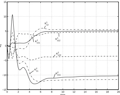
Kij

K1_z11

K2_z11 K1_z12

K2_z12

K2 11

K1 12

Fig. 5. Feedforward coordinated controller gain re-sponses

better than that with the standard adaptive laws (Gavel and Šiljak, 1989).

8. CONCLUSION

In this paper, we have developed coordinated decen-tralized output adaptive controllers for a class of large-scale systems with unknown interconnected strengths. We presented a modified DMRAC scheme which re-quires an exchange of signals between the

differ-ent reference models, but does not involve the ex-change of output signals between the different subsys-tems. Our scheme can be classified as a decentralized adaptive control scheme with model coordination. It can not only guarantee closed-loop stability but also asymptotic zero tracking errors when uncertainties are present in the subsystems and interconnections. Since the reference model signals can be exchanged between the subsystems off-line before the operation of the sys-tem, this scheme is feasible. The local control laws are the same as those found in the literature. The proposed control structure can be viewed as an upgrade of exist-ing schemes.Simulation results show the effectiveness of our proposed scheme.

REFERENCES

Gavel, D. T. and D. D. Šiljak (1989). Decentralized adaptive control: structural conditions for sta-bility. IEEE Transaction on Automatic Control 34(4), 413–426.

Ioannou, P.A. and P. Kokotovich (1983). Adaptive Systems with Reduced Models. Berlin.

Jain, S. and F. Khorrami (1997). Decentralized adap-tive control of a class of large-scale nonlinear systems. IEEE Transaction on Automatic Control 42(2), 136–154.

Mirkin, B.M. (1986). Optimization of Dynamic Systems with Decentralized Control Structure. Frunze, (in Russian).

Mirkin, B.M. (1995). Decentralized adaptive control with model coordination for large-scale time-delay systems. In: Proc. 3rd European Con-trol Conference ECC-95. Vol. 4 of 4, part 1. pp. 2946–2950. Roma, Italy.

Mirkin, B.M. (1999). Adaptive decentralized control with model coordination. Automation and Re-mote Control 60(1), 73–81.

Mirkin, B.M. and M. Choi (1991). Adaptive Decen-tralized Control of Dynamic Systems. Bishkek, (in Russian).

Narendra, K.S. and A.M. Annaswamy (1989). Stable Adaptive Systems. New York.

Ortega, R. (1996). An energy amplification condition for decentralized adaptive stabilization. IEEE Transaction on Automatic Control 41, 285–289. Wen, C. and Y.C. Soh (1999). Decentralized model