R E S E A R C H A R T I C L E
Open Access
An unstructured immersed finite element
method for nonlinear solid mechanics
Thomas Rüberg
1,2*, Fehmi Cirak
3and José Manuel García Aznar
1*Correspondence: [email protected] 1Multiscale in Mechanical and Biological Engineering (M2BE), University of Zaragoza, María de Luna 3, 50018 Zaragoza, Spain Full list of author information is available at the end of the article
Abstract
We present an immersed finite element technique for boundary-value and interface problems from nonlinear solid mechanics. Its key features are the implicit
representation of domain boundaries and interfaces, the use of Nitsche’s method for the incorporation of boundary conditions, accurate numerical integration based on marching tetrahedrons and cut-element stabilisation by means of extrapolation. For discretisation structured and unstructured background meshes with Lagrange basis functions are considered. We show numerically and analytically that the introduced cut-element stabilisation technique provides an effective bound on the size of the Nitsche parameters and, in turn, leads to well-conditioned system matrices. In addition, we introduce a novel approach for representing and analysing geometries with sharp features (edges and corners) using an implicit geometry representation. This allows the computation of typical engineering parts composed of solid primitives without the need of boundary-fitted meshes.
Keywords: Immersed finite elements, Nonlinear solid mechanics, Nitsche’s method, CSG modelling, Cut-element stabilisation, Implicit geometry
Background
Conventional finite element methods (FEM) are an irreplaceable tool for the numerical analysis of a variety of physical and engineering problems. They rely on a conforming mesh which approximately matches the domain boundary and material interfaces. For this reason, mesh generation is an essential part of the workflow in FEM-based analyses [1]. Although the procedure is well-established, often the use of a boundary-conforming mesh can be limiting or even prohibitive. Fluid-structure interaction, large elastic deformations and shape optimisation are some applications where mesh entanglement can cause severe difficulties for conventional FEM.
In the last two decades or so, a number of finite element-based numerical methods have been introduced in order to eliminate the need for boundary-conforming meshes. Here, we restrict ourselves to immersed methods, also known as embedded of fictitious domain methods, that operate with a geometry-independent mesh, in the line of [2–6]. Since the mesh of an immersed domain method does not conform with the boundary of the physical domain, one of these methods’ main difficulties is the application of boundary conditions. Here, we choose Nitsche’s method [7] for the weak enforcement of Dirichlet boundary conditions because it gives optimal convergence rates without incurring major
©2016 The Author(s). This article is distributed under the terms of the Creative Commons Attribution 4.0 International License (http://creativecommons.org/licenses/by/4.0/), which permits unrestricted use, distribution, and reproduction in any medium, provided you give appropriate credit to the original author(s) and the source, provide a link to the Creative Commons license, and indicate if changes were made.
implementation difficulties. Moreover, the use Langrange multipliers together with its numerical intricacies, such as the fulfilment of the LBB-condition [8], are avoided. For alternative approaches, see [4,9–14] among others.
A major difficulty of non-body-fitted methods is the accurate integration of the aris-ing volume and surface integrals. Here, we make use of a tessellation concept which allows to incorporate standard, Gauß quadrature schemes. In the course of this develop-ment, a technique is presented which enables the representation of sharp domain features by performing constructive solid geometry (CSG) modelling directly on the embedding mesh. This approach poses a clear advantage in comparison to the conventional methods of geometry resolution because these sharp features are accurately reproduced and not chamfered even on coarse meshes.
Another pitfall of immersed finite element methods is the loss of numerical stability in cases where the intersection of a shape function support with the physical domain becomes very small. This issue has been successfully addressed in the context of b-spline finite ele-ments [6,12,15]. In this work, we build up on this concept of constraining critical degrees of freedom and apply it to Lagrangian basis functions on unstructured meshes. Note that Burman et al. [16] introduced an alternative approach, the so-calledghost-penalty stabili-sation method, which is based on an augmented bilinear form. Strongly related to stability are the method’s parameters and we show how to choose these parameters in the context of the introduced stabilisation techniques.
The method we present here is based on our previous works [6,17–19] and related to [2,3,16,20,21]. Although, as shown in the cited works, the method can be transferred to many physical applications, we focus on the problem class of nonlinear elasticity.
Weak enforcement of boundary and interface conditions
At first, we present the derivation of the proposed immersed finite element method as applied to boundary value problems from nonlinear solid mechanics. Using a weighted residual technique, we obtain the weak form of the problem and give its linearisation. Similarly, the expressions for material interface problems are subsequently derived.
Boundary value problems of nonlinear solid mechanics
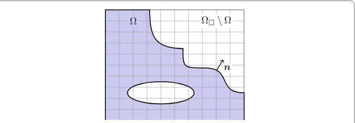
Consider the boundary value problem for nonlinear elasticity in the reference domain ∈Rnd,nd=2 ornd=3 (Fig.1)
n
Ω Ω \Ω
−Div P(u) =f in
u =u¯ onD
t(u)=t¯ onN,
(1)
whereudenotes the unknown displacement field,Pis the first Piola-Kirchhoff stress ten-sor, Div is the divergence with respect to reference domain coordinates, andt(u)=P(u)n, withnthe outward unit normal vector to, is the boundary traction. The prescribed data are the volume forcef, the prescribed displacement ¯uand the prescribed traction ¯t. The boundary of, denoted by, is composed of disjoint sets, the Dirichlet boundaryDand
the Neumann boundaryN, where the respective data are given.
In order to construct a weak form of the boundary value problem (1), a weighted residual approach is taken with the test functionv. In mathematical terms, we operate with the Sobolev spaceH1(), i.e. the vector fields whose components are all inH1(), see, among others, [8] for the precise definition. Different from conventional FEM, we do not employ a constrained subspace with essential boundary conditions. The weighted residual method thus becomes:
Findu ∈H1() R(u,v)=a(u,v)−
f ·vd−
N
¯
t·vd−
D
t(u)·vd=0
∀v∈H1(), (2)
with
a(u,v)=
S(u) : ˙E(v)d. (3)
Here, ˙Edenotes the variation of the Euler-Green strain tensor (E= 12(FF−I) with the deformation gradientF) andS=F−1Pthe second Piola-Kirchhoff stress tensor [22,23]. In the applications section, we work with a compressible Neo-Hooke material with given energy densityW(E) and for this hyperelastic case, the stress tensor becomes
S= ∂∂WE . (4)
Using a Newton method to solve the nonlinear Eq. (2), thekth iteration takes the form
DR(u(k),v)[u]= −R(u(k),v) and u(k+1)=u(k)+u, (5) where D(·)[u] denotes the derivative in direction of the incrementu, which reads
DR(u,v)[u]=Da(u,v)[u]−
D
Dt(u)[u]·vd (6)
with
Da(u,v)[u]=
(Gradv) : ˆC(u) : (Gradu)d. (7)
In this expression, ˆCdenotes theeffectiveelasticity tensor [22]. For simplicity, it is assumed here that the prescribed volume and surface forces,f and ¯t, are independent of the dis-placementu(dead load case). If these assumptions do not hold, the directional derivative ofR(u,v) contains the derivatives of the applied force and traction terms. So far, expres-sions (2) and, consequently, (5) do not take into account the displacement boundary conditionu = u¯ onD. Therefore, the approach initially introduced by Nitsche [7] is
adapted here and the following two terms are added to (5)
−
D
Dt(u)[v]·(u−u˜)d and γ
D
with the predictor ˜u=u¯in the first iteration (or the appropriate value in the first iteration of every load step) and ˜u=0otherwise, corresponding to a displacement-controlled New-ton method. The scalarγ >0, necessary for numerical stability, is discussed in “Numerical stability” section. In summary, the Newton step (5) including Nitsche’s approach to incor-porate displacement boundary conditions reads
Da(u,v)[u]−
D
Dt(u)[u]·vd−
D
Dt(u)[v]·ud
+γ
D
u·vd = −a(u,v)+
f ·vd+
N
¯
t·vd
+
D
t(u)·vd−
D
Dt(u)[v]·u˜d+γ
D
˜
u·vd, (9)
where the iteration counter has been omitted for sake of legibility. The added terms (8) are zero for the exact solution and therefore the method is consistent by construction. Moreover, for hyperelastic materials expression (9) is symmetric and positive for the right choice of γ and non-softening material behaviour, see “Numerical stability” section. In the following, we abbreviate (9) by
A(u;u,v)=(u;v). (10)
Material interfaces
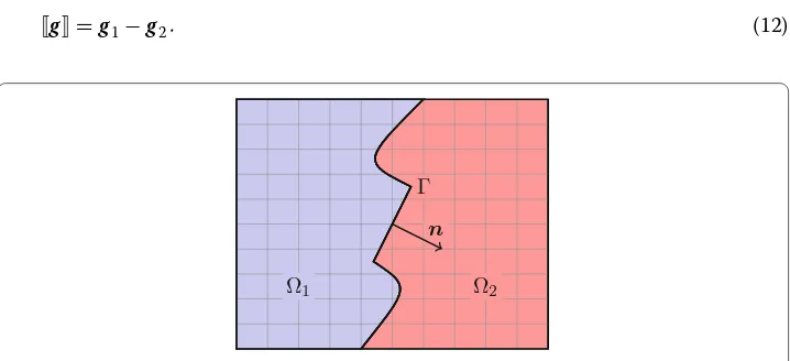
The formalism presented above for the weak incorporation of displacement boundary conditions can be generalised to interface problems, see also [2,3,13]. For simplicity, let the reference domain be composed of two subdomains,=1∪2, and let us ignore the
Dirichlet boundary conditions on∂. The treatment of such conditions is here essentially the same as in “Boundary value problems of nonlinear solid mechanics” section. We focus only on the conditions imposed on the material interface =∂1∩∂2, see Fig.2. In
each subdomainithe local equilibrium reads
−DivPi(ui)=fi ini. (11)
Let u denote the compound displacement field, such that u|i = ui, and define the
compound test functionvsimilarly. Moreover, for any compound functiong, withg|i=
gi, the jump acrossis denoted with
g=g1−g2. (12)
n
Ω1 Ω2
Γ
For later use, also a weighted average{g}is defined onas
{g} =βg1+(1−β)g2, (13) where 0≤β≤1 is some weighting parameter yet to be discussed. On the interfacethe conditions are
u=u and t(u)=t, (14)
with prescribed jump functionsu andt. These conditions represent the jump in the solid displacements and the traction equilibrium across the interface. In more complex situations, such as soft interfaces, a cohesive law can be imposed relating the interface tractiont to the displacement gapu, see [24]. Here, we assume thatu andt are prescribed and that they are independent of the displacementu. Note that in the evaluation of the tractionsti the unique normal vectorn = n1 = −n2as shown in Fig.2is used,
where this choice is arbitrary.
Repetition of the steps as in the single-domain problem above yields the weighted residual method for interface problems
Findui ∈ H1(i) i=1,2,such that
R(u,v)=
i=1,2
ai(ui,vi)−
i
fi·vid
−
t(u)·vd=0
∀vi∈H1(i). (15)
Now the integrand of the interface term is rewritten as follows
t(u)·v=[βt1(u1)+(1−β)t2(u2)]·v+[(1−β)v1+βv2]·t(u)
= {t(u)}v+[(1−β)v1+βv2]·t
(16)
employing the average term (13) and the interface conditions (14)2. Using a Newton
method to solve the nonlinear problem (15) with (16) requires the directional derivative
DR(u,v)[u]=
i=1,2
Da(ui,vi)[ui]−
{Dt(u)[u]} ·vd. (17)
The interface condition (14)1is now incorporated by adding terms akin to (8), namely
−
{Dt(u)[v]} ·(u−u˜
)d and γ
(u−u˜
)·vd, (18)
to expression (17). Again, the parameterγ >0 is yet to be discussed in the Appendix A and we use the predictor ˜u=uin the first iteration and zero afterwards. In summary, a step in a Newton iteration to solve the coupled interface problem reads
i=1,2
Dai(ui,vi)[ui]−
{Dt(u)[u]} ·vd−
{Dt(u)[v]} ·ud
+γ
u·vd=
i=1,2
i
fi·vid−ai(ui,vi)
+
{t(u)} ·vd
−
{Dt(u)[v]} ·u˜
d+
(1−β)v1+βv2
·td+γ
u˜
·vd. (19)
Immersed finite element method Finite element discretisation
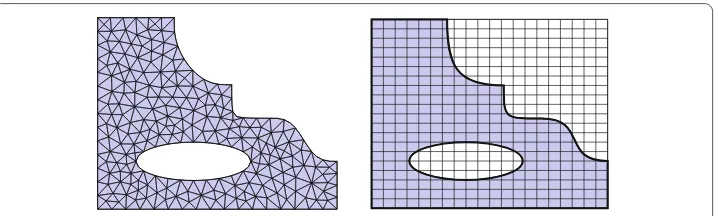
The linearised weighted residual Eqs. (9) and (19) form the basis of a finite element dis-cretisation. To this end, a domainof a simple shape, typically rectangular, is defined such that it fully contains the reference domain. The following finite element discreti-sation is based on a triangulation of instead of a geometry-conforming mesh of itself (see Fig.3). We use piece-wise polynomial basis functionsϕI(x) and write for the
approximated displacement field
uh(x)=
I
uIϕI(x). (20)
There is no constraint on the chosen finite element space, but if the surfaceoverlaps with the boundary of the embedding domain (that is if=∩∂= ∅), it can be more con-venient to use an essential treatment of displacement boundary conditions [8] along this boundary. On the other hand, if non-nodal basis functions (like, for instance, higher-order b-splines) are used as the finite element basis, the above presented weak incorporation of the boundary conditions works perfectly well on this boundary parttoo.
Let the support of the basis functionϕI be denoted by supp(ϕI). Now all coefficients
uI from the approximation (20) are discarded a priori if supp(ϕI)∩ = ∅. By Swe
denote the set of the indices of the remaining coefficients and thus{ϕI}I∈S forms the full basis of the immersed finite element method. This basis is in general not stable [25] and requires further attention, which is given in “Numerical stability” section. Using the approximation (20), we reach the final system of equations
Ax=b (21)
with the matrix and vector coefficients
A[I nd+a, J nd+b]=A(u;ebϕJ,eaϕI)
x[J nd+b]=(uJ)·eb (22)
b[I nd+a]=(u;eaϕI)
for the zero-based indicesI, J ∈ S, and using the coordinate directions 0 ≤ a, b < nd
(ndbeing the spatial dimension of the problem) and Cartesian unit vectorsea. Although
this immersed finite element method seemingly leads to the same type of linear system as a conventional, geometry-conforming FEM, there are technical differences which will be discussed in the following: the representation of the boundary or interface , the quadrature of elements traversed by this boundary, and the stabilisation of the basis for
such elements. The choice of the Nitsche parametersγandβis analysed in the Appendix A.
Above expressions hold analogously for interface problems. The main difference is that the two fieldsu1andu2are approximated in fashion of (20) independently on the same
background mesh ofwhich encompasses both sub-domains1and2. Consequently,
the elements which are traversed by the material interface approximate both fields since the FE shape functions of the entire element are used even though the fields are only defined up to the interface on their respective side of the domain. Using two sets of shape functions on these elements allows us to represent a discontinuous derivative of the FE solution and can thus be compared to the element enrichment of XFEM [11]. A good illustration of this implementation detail can be found in [2].
Signed distance functions
The weak forms introduced in “Weak enforcement of boundary and interface conditions” section allow us to work with a finite element discretisation which is independent of the geometry, but still the volume and surface integrals,(·)dand(·)d, need geometry information. To this end, we classify the elements (for instance the quadrilaterals in the right picture of Fig.3) by their location with respect to the physical domain. IfτIdenotes
any such element, we have the three cases:
1 τI∩= ∅, the element is completely outside ofand can be ignored,
2 τI∩=τI, the element is completely inside and its treatment is straightforward as
in any geometry-conforming FEM,
3 τI∩= ∅, the element is traversed by the domain’s boundary and requires special
consideration.
Note that elements adjacent to the boundary of the embedding mesh (for instance the left or bottom boundaries in the right picture of Fig.3) technically fall into the third category, but do not pose any difficulty apart from the identification of the element faces which lie on that boundary.
For above classification it is sufficient to have an oriented representation of the surface = ∂. Therefore, the surface is either closed or assumed to be extended beyond the boundaries of. Here, we assume thatis either given analytically or is approximated by means of a surface mesh composed of surface elementsσJ,
≈h=
J
σJ. (23)
In order to avoid the tedious task of intersecting volume elementsτIwith surface elements
σJ, an implicit geometry representation is introduced. Therefore, the signed distance
function [26] is used which is defined as
dist(x)=s(x) min
y∈|x−y|, with s(x)=
⎧ ⎨ ⎩
1 ifx∈
−1 ifx∈/. (24) In case of interface problems as introduced in “Material interfaces” section, the above definition ofs(x) refers to1and2instead ofand its complement\. If is represented by a meshh, the signed distance function disthwith respect to this mesh
disth(x)=
K
dKϕK(x) withdK =dist(xK), (25)
whereϕK are the nodal finite element shape functions (not necessarily the same as in the
approximation (20)) and the coefficientsdK represent the value of the signed distance at
the finite element nodesxK.
The representation (23) can be of higher polynomial degree, given by NURBS patches [1,14,27] or subdivision surfaces [28,29]. But the computation of the coefficientsdKin (25)
and the quadrature described below are non-trivial tasks if theσJ have a degree higher
than linear simplex elements (straight lines in two or flat triangles in three dimensions). In that case, the computation of the distances dK requires the solution of nonlinear
equations, see, for instance, [30]. In the rest of this work, theσJare always linear (nd−
1)-simplex elements. Moreover, once only piece-wise linear elements are used for the surface representation (23), the optimal convergence rate of any higher-order method is impeded by this geometry approximation error, see [8].
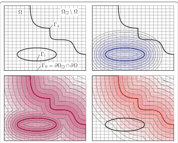
Figure4shows a two-dimensional example where the boundary is composed of three parts:0is the part of the boundary ofthat coincides with the box boundary∂and does not require any special attention;1and2are separated parts which are immersed
in the background grid. For the computation of the distance function dist, it is convenient to treat1and2separately as shown in the figure. The final distance function is then
composed as the minimal value of these distances,
dist(x)=mindist1(x),dist2(x). (26)
Ω \Ω
Ω
Γ0=∂Ω ∩∂Ω Γ1
Γ2
See also [31] for arithmetic with distance functions. Figure4 shows the iso-curves of the individual distance functions disti as well as of the composite function dist. The extension of this approach to a larger number of immersed surfaces is straightforward.
Once the function dist has been determined, the above classification of volume ele-mentsτI is carried out by means of the nodal valuesdK of the distance function: if all
dK of the elementτIare strictly positive (negative), the element is inside (outside) of the
domain. If a change in sign of thedKoccurs,τIis traversed by the immersed boundary.
It remains to outline how the coefficientsdKfor a given surface are computed. In case of
an analytic surface representation by an implicit function, these coefficients are calculated directly. In case of an immersed surface mesh, one needs to find the surface elementσK∗ which contains the pointx∗K closest toxK, see for instance [32] for such basic primitive
tests as the closest point on a triangle to a point. With the knowledge of the closest element σ∗
K, it can be decided ifxKlies on the positive or the negative side of this element in order
to determine the signs(xK) as defined in (24). This decision is based on the premise that
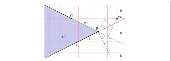
the surface mesh is well oriented. Note that, when the closest point falls on an edge or a vertex, ambiguities can arise for the decision if a point is inside or outside the surface mesh [26], see the case shown in Fig.5.
At the acute corner in the figure, the region of points whose closest point is the vertex B, is delimited by the outer cone. For all points in this cone,σ1andσ2are possible choices as
closest surface element. The cone contains the region ‘a’ in which the points are all outside with respect to both elements. The points in region ’b’ are outside with respect to one of the possible closest surface elements and inside with respect to the other. Hence, for this region the mentioned ambiguity can occur. One solution to this problem is to introduce angle-weighted vertex normal vectors [26], but this requires extra data structures. Here we choose the simpler approach shown in Fig.5: the pointxK has a larger distance to the
extension plane ofσ2than to the extension plane ofσ1. This distance is given by the inner
product of the element normal vector and the distance vector between the considered grid point and the closest surface point (here, B). Choosing the element with a larger value of this distance resolves the ambiguity. The method is also used in three dimensions with the only difference being a larger set of candidates as closest elements.
Finally, we consider the numerical complexity of the distance function computation. If there areNelements in the surface mesh andNnodes in the volume mesh, a
brute-xK
σ1 σ2
B
A C
b
a
b Ω
force approach requiresN×Nclosest point computations. In many cases, this number can be substantially reduced by precomputing a bounding box [32] of the surface h and assigning a default value for thedK of nodes outside of this box, but the essential
complexity remains of order O(N×N). Complexity reduction is possible by gener-ation of a hierarchy of bounding boxes [32] or using so-calledmarching methods, see e.g. [33].
Constructive solid geometry modelling
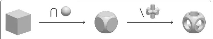
Now, we consider a different approach for integrating finite element analysis with geomet-ric design, similar to the ideas presented in [34]. Specifically, we consider the construction of a three-dimensional geometry by means of CSG, see, for instance, [35,36]. An example of such a modelling process is given in Fig.6, where one begins with a cube as a workpiece and performs set operations with other geometric primitives until the desired geometry is obtained. These operations are commonly union∪, intersection∩, subtraction\and the set complement (). Based on De Morgan’s laws [36], it suffices to work with the canonical operations intersection and complement, and represent the other two as compositions thereof, more preciselyA∪B=(A∩B)andA\B=A∩B.
The conventional finite element approach is to work through such a CSG pipeline, export a geometry representation and use a mesh generation software to create a body-fitted volume mesh for the numerical analysis. The direct modification for an immersed finite element method is to export a surface representation of the geometry and embed this into the mesh by the methods described in “Immersed finite element method” section. Here, a third way is suggested in which the set operations are directly applied to the embedding (non-conforming) volume mesh. As outlined above, it suffice to provide the complement and intersection operations only. The former is trivially achieved: the use of a signed distance function generates an in- and an outside partition of the mesh, reversing these partitions gives the complement. For this reason, all that need be explained is the intersection operation.
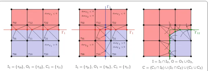
A simple two-dimensional example in Fig.7demonstrates the intersection operation: first the intermediate domain1is given via the distance function of a straight line1,
afterwards a second distance function to the line 2yields the final domain = {x ∈
: dist1(x) > 0 and dist2(x) > 0}. For sake of clarity, let us discuss the individual steps in this picture. First the line1is embedded into the shown 3×3-grid which fills
out the square domain. The elementsτi0are strictly inside the intermediate domain
1= {x ∈: dist1(x)>0}and form the setI1. The elementsτi2are strictly outside and form the setO1. Now, the remaining elements form the setC1and are triangulated
such that the embedded boundary is approximated by triangle edges. The squares are first
Γ1
distΓ1<0
distΓ1>0
τ00 τ01 τ02
τ10 τ11 τ12
τ20 τ21 τ22
I1={τi0},O1={τi2},C1={τi1}
Γ1
Γ2
distΓ2<0
distΓ1<0
distΓ1>0
distΓ2>0
distΓ1<0
distΓ2<0
τ00 τ10 τ01 τ11 τ02 τ12 τ22
τ20 τ21
I1={τ2i},O1={τ0i},C1={τ1i}
Γ12
I=I1∩I2,O=O1∪O2,
C= (C1∩I2)∪(I1∩C2)∪(C1∪C2)
Fig. 7 Intersection process. Domain partitioning and element tessellation for a straight boundary1(left), resulting constellation for intersection with another line2(middle); for comparison see the result of the immersion based on the composite distance function (right)
subdivided into two triangles each and then every such triangle is intersected by means of the nodal values of the signed distance function dist1[37]. The resulting outcome is the left picture in Fig.7where the red square-shaped marks indicate the location of the intersection points.
In the second embedding step, the distance function dist2 is used which gives rise to the element sets I2, O2 andC2. All elements which belong to the outside are directly
assigned to the complementary domain \, that is O = O1∪O2. On the other
hand, all elements of I1, which also belong toI2, are inside the final domain, hence
I=I1∩I2= {τ20}. Finally, there are the intersection cases. Elements belonging toC1and
I2(τ21) keep their status and sub-division. Elements fromI1andC2(τ10) are subject to the
same decomposition methods asC1. It remains to discuss the situation of the elements
which belong toC1∩C2; the ones which are intersected by both boundaries, and in our
example of Fig.7this is the elementτ11. In this case, simply the composing triangles are
intersected with2as if they were elements of their own. Proper categorisation of these
simplex shapes defines the final domainand its complement \, see the middle
picture of Fig.7.
The advantage of this approach becomes clear when looking at the right picture of Fig. 7. Shown is the result for the same target domain, but first the composition of the individual distance functions disti is computed according to expression (26) and then the element intersections are constructed. Clearly, in the right picture the corner is chamfered whereas in the above outlined approach this geometric feature is preserved. This is the distinctive characteristic of the presented idea: by successively embedding the geometry primitives into the mesh, the sharp features at the primitive intersections are preserved. It is important to remark that the boundariesihave been represented exactly
in this example, but this is solely owed to the fact that they are straight lines. In the more general situation of curved boundaries, they are again represented on the finite element mesh by piece-wise linear simplex elements. But, even though these surrogate boundaries do not exactly reproduce the given geometry, the here presented approach still allows to represent corners or edges at the intersection locations of the original primitives which lie inside of the finite elements.
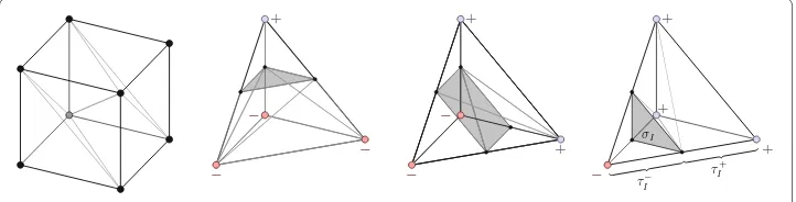
elements are subdivided into two triangles which themselves are triangulated in order to recover the implicit surface in the form of triangle edges. This approach is akin to a two-dimensional version of marching cubes and in three dimensions we make use of a similar technique. The used three-dimensional element shapes are either tetrahedrons or hexahedrons. Figure8shows how a hexahedron is decomposed into six tetrahedrons such that it remains to consider this shape only. Given a tetrahedron with values of the signed distance function at its vertices we can classify the cases shown in the right part of the figure. Based on linear interpolation along the edges the zeros of the distance function are recovered and give rise to two volume tessellationsτI−andτI+whose common faces form the triangulated surfaceσI. Using these decompositions, the above outlined
inter-section operations of two geometry primitives can be carried out analogously in three dimensions.
Alternative approaches for increasing the quality of implicit geometry representations in the vicinity of sharp features (such as edges and corners) exist. In [38] the operations of surface reconstruction by means of marching cubes and the distance function com-putation are combined in order to generate a so-called directed distance field allowing for a better resolution of surface features. On the other hand, enriched distance func-tions are presented in [39] where additional edge and vertex descriptors augment the distance geometry representation. Although both approaches are promising concepts in the context of immersed finite element methods, they are not further considered in this work.
We conclude this paragraph by noting that the here used tessellation techniques also help to construct numerical integration schemes for the elements that are traversed by the boundary or interface. The cut elements are general polytopes for which quadrature rules are not easily obtained. There are many techniques that address this problem, such as moment-fitting [40], surface-only integration [41], and adaptive decomposition of the integration region [14,42]. But since we have a tessellation in simplex shapes already available, we use composite Gauß type quadrature rules, see e.g., [11].
Numerical stability
Up to now, it has been shown how to derive an immersed finite element method for boundary value and interface problems, see (9) and (19), and how to compute the matrix coefficients of the linear system of equations. But the stable solution of this final system of Eq. (21) remains to be discussed, especially in view of the method’s parametersγ (for boundary value and interface problems) andβ(for interface problems only).
−
−
+
−
−
+ +
−
−
+ +
+
τ−
I
τ+
I σI
Sources of instability
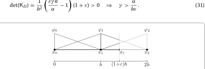
As an illustrative example, consider a one-dimensional problem
−αu =f x∈(0, xε)
u=0 x=0 (27)
αu=0 or u=0 x=xε
for the domain=(0, xε) and a constant material parameterα. The boundary conditions are a prescribed value ofu=0 at the left end and either a zero derivative (homogeneous Neumann) or a zero function value (homogeneous Dirichlet) at the right end. Let = (0,2h) be the embedding domain and two linear finite elements of sizehare used for the discretisation, see Fig.9. First, we consider the case with a homogeneous Neumann boundary condition at the right end. The left-side boundary condition is going to be incorporated essentially and the system matrix becomes
KN = α
h
1+ε −ε
−ε ε
. (28)
Obviously, for ε → 1 this matrix recovers the standard finite element matrix for this problem with its known properties. The eigenvalues of this matrix have the values
λ1,2= α
2h
1+2ε±4ε2+1. (29)
Clearly, the smaller eigevalue goes to zero for the limitε→0, that is the case of a vanishing cut element. As expected, the matrixKN is ill-conditioned for this limit.
We now turn to the Dirichlet case and evaluate the left-hand-side of expression (7) for this simple test problem. The resulting stiffness matrix has the form (replacing the surface integrals by point evaluation atxε)
h αKD=
1+ε −ε
−ε ε
−
ε−1 1−ε
−ε ε
−
ε−1 −ε
1−ε ε
+γhα
(1−ε)2 ε(1−ε)
ε(1−ε) ε2
. (30)
Note that the expression for the system matrix has been multiplied by the factor hα. The expressions of the eigenvalues of KD are not easily determined, but the condition
det(KD) > 0 is more workable. Note that since the trace of the matrix is positive and
equalsλ1+λ2, the condition of a positive determinant (recall det(KD)=λ1λ2) is sufficient
for positive definiteness. One gets
det(KD)=
1 h2
εγ h
α −1
(1+ε)>0 ⇒ γ > α
hε. (31)
0 h (1+ε)h 2h
x0 x1 xε x2
ϕ0 ϕ1 ϕ2
Fulfilment of this condition guarantees that the matrix is positive definite for a fixed mesh sizeh, but unfortunately it impliesγ → ∞forε→0. The use of a very large value forγ can lead to undesired numerical problems.
In the case of the interface problems and formulation (19), the situation is slightly better. The extra parameterβcan be adjusted in a smart way such that a finite value ofγis always achievable. Such a choice is proposed in [43] whereβdepends on the material parameters of the subdomains and the sizes of the cut elements,|τI∩i|. Using this approach, the
system matrix has always positive eigenvalues (for the considered problem class) with a finite value ofγ. Nevertheless, the minimal eigenvalue goes to zero for vanishing sizes of the cut elements. Even though the parameter choices by [43] show a good performance in terms of the quality of the numerical results, the matrix condition number still cannot be bounded for a fixed mesh and arbitrary interface locations.
Stabilisation
The above indicated sources of numerical instability all stem from the same situation that for some degrees of freedom, the intersection of the support of their associated shape functions with the physical domain becomes very small,
sI= |supp(ϕI)∩| h , (32)
where supp(ϕI) denotes the support of shape functionϕIandhis a measure of the mesh
size on. In all above cases, Neumann, Dirichlet, or interface problem, this leads to severe ill-conditioning of the final system matrix. To solve this problem, the following approaches have been proposed, among others,
S-1 Discarding all degrees of freedom with support intersection below a certain thresh-old,sI< εh;
S-2 Adding a face-based stabilisation term [16]; S-3 Constraining degenerate degrees of freedom [6,12].
As reported, among others, in [12], the approach S-1 leads to a loss of approximation order. Although appealing due to its simplicity, this drawback can be prohibitive in some applications. An ad-hoc approach to remedy the stability problem is to locally adapt the finite element mesh in order to avoid the problem of too small values ofsI. Even though
simple at first sight, a robust realisation of this idea in three dimensions is not straight-forward and mesh entanglement needs to be avoided. The support sizesIis increased if
specific nodes are moved away from the surface, but there is an interesting alternative in which the points are snapped to the surface thereby generating a conforming mesh, see [44] for two-dimensional analysis of this idea.
this factor the stabilisation effect disappears and for too large values the method’s accuracy is affected [16].
Finally, we consider S-3 which relies on the concept of coupling degrees of freedom with too small supports to other degrees of freedom from the interior of the domain. In order to outline this approach, the degrees of freedom shall first be classified according to the sizesIof the intersection of their support with the domain, as defined in (32). In “Finite
element discretisation” section, the setShas been introduced which contains all indices of shape functions for whichsIis larger than zero. Introducing a threshold ˆs, the setSis
now decomposed into the disjoint index sets,AandBwith definition
A= {I ∈S:sI ≥ˆs} and B= {I∈S:sI <ˆs}. (33)
The threshold ˆsused in this classification has to depend on the mesh sizehand should not be larger than one typical element size. The basic idea of Höllig et al. [12] is to constrain degrees of freedom from the set Bto suitably chosen degrees of freedom fromA(J), a subset ofA,
∀J∈B: uJ =
I∈A(J)⊂A
cIJuI (34)
where the coefficientscIJ will be discussed further below. These constraints give rise to
the modified shape function basis
uh(x)=
I∈A
uIϕI(x)+
J∈B uJϕJ(x)
=
I∈A
uIϕI(x)+
J∈B
⎛
⎝
K∈A(J)
cKJuK
⎞ ⎠ϕJ(x)
=
I∈A uI
⎛
⎝ϕI(x)+
J∈B(I)
cIJϕJ(x)
⎞ ⎠=
I∈A
uIϕ˜I(x). (35)
In this reordering of the finite element approximation (20) a new setB(I) is used which contains all indicesJ fromB, such thatI ∈ A(J). For the implementation of this sta-bilisation method, it is sufficient to work with expression (34), but the result of (35) demonstrates that effectively a modified shape function basis {ϕ˜I}I∈A is generated and
illustrates the notion of extended splinesas given in [12]. Note also thatB(I)= ∅for all degrees of freedom that are not in the vicinity of the boundary and in that case ˜ϕI =ϕI,
so that most shape functions are not affected. Since the support size of the basis functions ˜
ϕI is larger, the bandwidth increases for these degrees of freedom. Therefore, it has to
be remarked that only degrees of freedom in the vicinity of the boundary are affected. Moreover, the storage requirement of the final system matrix is of course not larger than it would be for the original (unstable) basis functionsϕI.
There are two open questions when using this approach: (i) the choice of the index set
A(J) associated toJ and (ii) the values of the constraint weightscIJ. The origin of this
approach, as introduced in [12], is to stabilise b-spline discretisations. In this particular situation, the underlying mesh is logically Cartesian and an explicit expression of the coefficients cIJ can be given as a function of the multi-indices used to label that grid.
approximation quality of the approximation (20) due to the constraints (34). In other words, the modified basis functions ˜ϕI introduced in (35) have to represent the same
polynomials as theϕIthemselves.
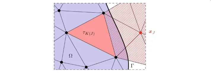
In order to outline the procedure for obtainingA(J) and the corresponding coefficients cIJ, consider the situation depicted in Fig.10. The degree of freedomuJ,J ∈ B, resides
at nodexJ and the size of the intersection of the support (hatched in the picture) with
the domainis below the threshold ˆs. Searching through the elements in the vicinity of
xJ, one finds the elementτK(J)whose connected degrees of freedom all belong toA. Any
element entirely inside the domainfulfils this condition. Normally, many such elements can be found and the closest is selected, where the distance between the element middle point andxJ is a possible way to measure the proximity. The selected elementτK(J)gives
rise to the index setA(J)⊂Aassociated withuJ. Formally, we can write
A(J)= {I∈A: supp(ϕI)∩τK(J)= ∅}. (36)
Once this set is defined, the weightscIJare calculated by evaluation of the basis ofτK(J)at
the nodexI,
∀I∈A(J) :cIJ =ϕI(xJ). (37)
This choice of weights is an extension of the idea given in [15] where the weights are defined for non-uniform b-splines as dual functionals applied to the polynomials in a chosen grid element. Here the point evaluation of (37) is the corresponding dual functional of Lagrange polynomials [8]. Note thatxJ ∈/τK(J)and thuscIJ represents an extrapolation
of the polynomial basis spanned in τK(J) to the outside point xJ, see also Fig. 10. The
stabilisation procedure can be summarised as follows
1 categoriseAandBusing a threshold ˆs, see (32) and (33) 2 for allJ∈B
• findτK(J)with all degrees of freedom fromAthat is close toxJ,
• define the constraint coefficients ascIJ =ϕI(xJ) for allI∈A(J)
3 assemble the final system of equations using the constraint equations (34) applied to test and trial spaces
4 after solving the global system, calculate the constrained degree of freedomuJ with
J∈Baccording to (34).
Γ Ω
xJ
τK(J)
Fig. 10 Cut-element stabilisation on a triangular mesh. NodexJis the location a degree of freedomuJ,
With respect to the implementation a few remarks have to be made. The code has to be able to search the elements in the neighbourhood of a given node. For instance, the elementτK(J)in Fig.10does not lie in the support ofϕJbut in the ring of elements around
that support. Theoretically, for very extreme shapes ofthe nearestτK(J)toxJ could lie
far away, but here we assume that the mesh is fine enough such that there is always an element nearby. Cusp-shaped domains are excluded from the onset. In addition, one has to evaluate the shape functions ofτK(J)atxJ and this requires to find first the reference
coordinateξJ (outside of the reference element) such that the geometry representation of the chosen element representsxJ when evaluated at this coordinate, that isxK(J)(ξJ)=xJ.
Here we restrict ourselves to meshes in which all elements are an affine transformation of the reference element. Higher-order geometry representations of the volume mesh are excluded, but they are also not necessary since the mesh, by design of the immersed method, need not conform to the geometry of.
Numerical examples
At last, a few numerical examples are presented in order to study and demonstrate the per-formance of the immersed finite element method as presented here. Unless indicated oth-erwise, the spatial discretisation of all problems is carried out with linear finite elements. As shown in the appendix, the Nitsche parameter is chosen asγ = γ0αh with the mesh
widthh, the representative material parameterαand a dimensionless scalarγ0. The default
choices for this parameter isγ0=10 and for interface problems the additional parameter
is chosen asβ=0.5. The threshold ˆsused to distinguish between the degree of freedom setsAandBin the stabilisation of “Stabilisation” section is set to the size of one element.
Convergence and robustness analysis
At first, the method’s performance under variation of various parameters is assessed. For this purpose, an essentially one-dimensional Poisson problem is used as depicted in Fig.11, left, with a forcing functionf(x)= α2sin(αx
1) andα = 23xπδ. The resulting exact
solution is thenu(x)=sin(αx1). The signed distance function is dist(x)= xδ−x1and
the boundary is represented exactly. At first, this problem is analysed using a structured mesh as shown in the figure. Figure11, on the right, shows the analytic solution (solid
x1= 0 xδx1= 1
∂2u= 0
∂2u= 0
−∂11u=f(x1)
u
=0
u
=¯
u
or
∂1
u
=0
0 0.2 0.4 0.6 0.8 1
−1
−0.5 0 0.5 1
xδ
coordinatex1
v
alues
o
f
u
and
∂1
u/α
u ∂1u/α exact h= 0.2 h= 0.1
black line) along the x1-axis and its derivative (dashed line) for a boundary location at
xδ = 67. The approximations uhand∂1uhfor a mesh with 5×5 elements (red) and a
10×10 element (blue) are also displayed. One can see that the numerical approximation uhcoincides with the analytic solution at the finite element nodes and, moreover, at the boundary location atxδ.
The convergence of the method is shown in the left of Fig.12, where the numerical errors inL2-norm andH1-seminorm are shown for an approximation with linear and a
quadratic Lagrange polynomials. These results exhibit the expected optimal convergence rates [8]. In this graph, the boundary location is held fixed atxδ= 67and the mesh width his decreased. On the other hand, the right side of Fig.12shows the smallest and largest eigenvalues of the system matrix in dependence of the boundary location for a non-stabilised implementation and for the stabilisation presented in “Stabilisation” section. Here, a fixed 40×40 mesh is used and the location of the boundary is atxδ =(34+ε)h with the parameter 0≤ε≤1. A Neumann boundary condition atxδis considered and, hence, one has alwaysa(uh, uh)>0 andλmin>0. One can clearly see thatλmin∈O(ε) for
smallεand for the non-stabilised case (note that the figure shows in fact the inverseλ1 min). Clearly, the matrix condition number grows without bound. The stabilisation as outlined in “Stabilisation” section, however, guarantees a constant value ofλminwell above zero.
The largest eigenvalues coincide for both cases.
Now we turn to the problem with a Dirichlet boundary condition atxδ. Using the same variation of the location of this boundary as above, Fig.13shows the smallest eigenvalue λminfor the stabilised method and for the non-stabilised method for various values of
γ0(recall thatγ = γh0). One can see that without stabilisation the considered minimal
eigenvalue changes sign for decreasing values ofεrendering the system matrix indefinite (and singular when the zero is crossed). In order to force λmin > 0 one can increase
the value ofγ0, but forε → 0 this value grows without bound and one gets effectively
λmax → ∞which likewise deteriorates the condition number of the matrix, as already
discussed in “Sources of instability” section.
Next, the stabilisation technique is applied to an unstructured mesh as shown in Fig.14. Note that this case is not covered by the original idea of this technique as given by [12] which was only designed for b-spline basis functions on structured meshes. The left of Fig.15shows the convergence of the stabilised method for linear triangle elements and
10−2 10−1
10−7 10−5 10−3 10−1
O(h)
O(h2)
O(h3)
element sizeh
appro
ximation
error
L2
H1
linear quadratic
10−9 10−7 10−5 10−3 10−1 100
102 104 106 108 1010
O(ε−1)
cut element sizeε
extremal
eigen
v
a
lues
1/λmin
λmax not stabilised stabilised
Fig. 12 Neumann problem. Convergence forxδ=6
10−9 10−7 10−5 10−3 10−1 −0.08
−0.06 −0.04 −0.02 0
cut element sizeε
eigen
v
alue
λmin stabilised,γ0= 10 not stabilised,γ0= 1000 not stabilised,γ0= 100 not stabilised,γ0= 10
Fig. 13 Dirichlet problem. Smallest eigenvalue for various boundary locations (h=0.025 and
xδ=(34+ε)h)
0.8 0.9 xδ
Fig. 14 Unstructured mesh. Varying location of the right boundary atxδ
a fixed boundary location. Finally, the location of the boundary is varied again and the condition number for a Neumann problem is considered in the right of Fig.15. Whereas in the non-stabilised case this value shows a very erratic behaviour with large peaks, the condition number for the stabilised method is almost constant at a low value.
Now, an interface problem is considered. Figure16shows the computational domain that is composed of a circular domain 1 embedded in a square domain2. On this
10−2 10−1 10−4
10−3 10−2 10−1 100
O(h)
O(h2)
element sizeh
appro
x
imation
error
L2
H1
0.8 0.82 0.84 0.86 0.88 0.9 103
104 105
boundary locationxδ
condition
n
um
b
er
|
λmax
/
λmin
| stabilisednot stabilised
Ω
1Ω
2L
R
10−2 10−1 10−3
10−2 10−1 100
O(h)
O(h2)
element sizeh
appro
ximation
error
β= 0 β= 0.5 β= 1.0 L2
H1
Fig. 16 Interface problem. Computational setup of a square with a circular inclusion (left), convergence behaviour for different interface weightsβ(right); note that these curves are not distinguishable
domain, the Poisson problem−αiu = 4 with material parametersα1 = 1 andα2 =
1000 is solved, subject to Dirichlet boundary conditions on the outer boundary∂2. The
geometric parameters are chosen as R = 0.75 andL = 2, respectively. This problem together with its analytic solution is taken from [2]. In the right graph of Fig. 16the convergence behaviour is shown for different values of the interface weight factorβ. For the three considered valuesβ =0, 0.5 and 1, the curves are indistinguishable. Also optimal convergence rates are achieved for mesh sizes smaller thanh≈0.02.
At last, we consider the influence of the geometry representation. As outlined in “Con-structive solid geometry modelling” section, we have to approaches available: the use of a signed distance function representing the entire embedded surface and the successive embedding of the geometry primitives that form the final model. For simplicity, consider a square that coincides on two of its edges with the mesh boundary whereas the other two are represented implicitly. Figure17shows the effect of the introduced two approaches in the left and middle images, respectively. Clearly, the upper right corner is chamfered off in the first approach, but represented exactly in the second. As a numerical problem we have chosen−u=1 on a unit square subject tou=0 on the lower and left boundaries and ∂u/∂n = 0 on the other two boundaries. An analytic solution to this problem is
10−2.5 10−2 10−1.5
10−6
10−5
10−4
10−3
O(h2)
element sizeh
L2
error
CSG fully implicit
available, for instance in [45] in the context of Poiseuille flow in a rectangular channel. The right graph in Fig.17shows the convergence rates for the two types of geometry modelling. Clearly, optimal convergence rates are obtained for both cases. Nevertheless the exact representation of the corner leads to a much smoother outcome with lower approximation errors for coarse mesh sizes.
Mesh-embedded CSG
Here the domain as obtained by the CSG process of Fig.6is reconsidered, see also the left of Fig.18. The embedding domain is=(0,1)3and equipped with a uniform hexahedral
mesh. Following the mesh-based Boolean operations as introduced in “Constructive solid geometry modelling” section, the immersed geometry is obtained by
1 intersectionwith a sphere of radius 0.65 and centred at (0.5,0.5,0.5), and
2 successivesubtractionof cylinders around the same centre with radius 0.3 and in the directions of thexi-coordinate axes.
Thus the domainis obtained as shown in Fig.18and we assume that it is occupied by a hyperelastic solid. In a first analysis, linearised elasticity is assumed and the convergence is studied by using fundamental solution of elasticityU(x,y) (see, for instance, [46]) as an imposed analytic solution with a source pointylocated outside of the domain. Therefore, on the bottom (x3 = 0) the boundary displacements ¯u(x)= U(x,y) are prescribed and
the remaining boundaries are subject to the Neumann condition ¯t = t(U)(x,y). For simplicity, the material parameters are chosen asλ=28.85 andμ=19.23. The right of Fig.18shows the convergence of the displacement solution and of the computed volume and surface area of the embedded domain. Quadratic convergence is observed for all considered quantities.
Next, a compressible Neo-Hookean material model [22,23] with large deformations is used, based on the strain energy density
W(F)= λ 2(logJ)
2−μlogJ+ μ
2(trC−3), J=detF and C =F
F, (38)
with the deformation gradientF = I+Gradu. The material parameters are the same as in the linearised case above. For the example, the bottom boundary is held fixed and a
0.05 0.1 0.2 0.0001
0.001 0.01 0.1
O(h2)
element sizeh
appro
ximation
errors
u−uh
|V−Vh|
|A−Ah|
twisting traction field is applied to the top surface with value ¯t=10(x2−0.5,0.5−x1,0).
The load is applied in 4 steps and within each step a Newton method is used to obtain the equilibrium state. The deformed geometry for these four load steps is shown in the images of Fig.19for a 403grid of linear hexahedron elements.
Composite material
As a last example, the elastic deformation of a fibre-reinforced block of elastic material is considered. A block of dimensionL×25L×Lis reinforced by inclined fibres placed with a main axis separation of L3. The fibres are represented by cylinders with radius 15L. The three-dimensional setup is shown in the left of Fig.20and on the right a two-dimensional view of the problem is depicted. The bottom surface is held fixed and the top surface is constrained in normal direction. The left and right surfaces are subject to a constant traction field ¯t in normal direction. The discretisation is carried out by a fixed mesh of dimension 50×20×50 as indicated on the back faces of the three-dimensional view. For comparison, we monitor the average horizontal displacement
U1=
1
||
u1(x)d (39)
throughout the composite body for a variety of fibre angles −35◦ ≤ α ≤ 35◦. Both domains1and2have the hyperelastic material law according to the energy (38) and
Fig. 19 Large elastic deformation. Load steps 1–4; the surface iscolouredby the stress componentS33
2/5L ¯t ¯t
α
Ω2 Ω1
L
L
L/3
R u·n= 0
u=0
−30 −20 −10 0 10 20 30 0.14
0.15 0.16 0.17 0.18 0.19
fibre angleα
a
v
erage
displacemen
t
U1
Neo-Hooke linearised
Fig. 21 Computational analysis of fibre-reinforced material. Deformed geometry with fibres coloured byS33 forα= −35◦(top left),α=0◦(top right), andα= +35◦(bottom left); average horizontal displacementU1 for various fibre angles (bottom right)
the computations are carried out with large deformations. For comparison, a linearised situation is also considered.
The model parameters are chosen asL =1 and ¯t = (1,0,0). The materials are repre-sented by the Lamé parametersλ1=5.769,μ1=3.846,λ2=10λ1andμ2=10μ1.
Fig-ure21shows the deformed configuration for fibre anglesα= −35◦,α=0◦andα= +35◦. In addition, the analysis of the average horizontal displacementU1as a function of the
considered fibre anglesαis shown for the Neo-Hooke material and linearised elasticity. Although there are similarities between the large-deformation analysis and the linearised version, striking differences can be observed too. Most of all, the linear variant is com-pletely symmetric with respect to the sign ofαand has its largest value forα=0◦. In the large-deformation variant, on the other hand the result is a larger deformation for the nega-tive fibre angles and smaller for posinega-tive angles. Overall, the body behaves less flexibly in the nonlinear analysis, but with a strong bias to an increased flexibility for negative fibre angles.
Conclusions
allow for more flexible geometry processing and remove the repeated interaction with mesh generation software. Here, we present an immersed FEM for the problem class of nonlinear elasticity, based on a weak incorporation of Dirichlet boundary conditions and interface conditions with Nitsche’s method, an implicit geometry representation and accurate integration of the arising cut elements. We place emphasis on the implementa-tion details such as the robust computaimplementa-tion of the signed distance funcimplementa-tion and quadrature by means of tessellation. A common pitfall of non-body-fitted FEM, the loss of numerical stability in situations with degenerate function support, is analysed and we provide a sta-bilisation technique that is robust without affecting the convergence behaviour. Moreover, the choice of the parameters in the context of Nitsche’s method are thoroughly discussed. We demonstrate a way to incorporate sharp features such as edges and vertices in our method by means of successively embedding the geometry primitives into the analysis mesh in a similar way as in constructive solid geometry modelling. Based on this idea, geometry modelling is directly integrated in the finite element analysis and there is no need for a mesh generation tool. The presented applications emphasise the potential of this approach, where large deformation analyses are carried out based on a trivial Cartesian background mesh.
A present shortcoming of the introduced approach is the restriction to linear approx-imation orders. Although the field approxapprox-imation used in this FEM can be of arbitrary order, a gain in convergence order would be impeded by the geometry representation based on linear facets. In principle, the use of more accurate signed distance functions and the subsequent adaptation on the quadrature level to account for embedded higher-order surface representations is feasible.
Finally, we note that the presented method is ideally suited for the incorporation ofh -adaptivity. A combination of this immersed FEM with hierarchical refinement techniques as shown, for instance, in [47] would render a powerful analysis toolbox, which yields accurate numerical predictions based only on the input of geometry primitives.
Authors’ contributions
The presented ideas are joint contribution of the three authors. TR implemented the numerical techniques and wrote the initial draft of the paper. JMGA and FC contributed to the revision of the draft. All authors read and approved the final manuscript.
Author details
1Multiscale in Mechanical and Biological Engineering (M2BE), University of Zaragoza, María de Luna 3, 50018 Zaragoza, Spain,2Institut für Baumechanik, TU Graz, Technikerstraße 4, 8010 Graz, Austria,3Department of Engineering, University of Cambridge, Trumpington Street, Cambridge CB2 1PZ, UK.
Acknowledgements
This work was partially supported by the EPSRC (second author, Grant #EP/G008531/1), by the European Research Council (third author, Grant #ERC-2012-StG 306751), and by the Spanish Ministry of Economy and Competitiveness (third author, Grant #DPI2015-64221-C2-1-R).
Competing interests
The authors declare that they have no competing interests.
Appendix A: method parametersγandβ