The Thirty-Third AAAI Conference on Artificial Intelligence (AAAI-19)
Asynchronous Delay-Aware Accelerated Proximal
Coordinate Descent for Nonconvex Nonsmooth Problems
Ehsan Kazemi,
1∗Liqiang Wang
11Department of Computer Science, University of Central Florida
ehsan [email protected], [email protected]
Abstract
Nonconvex and nonsmooth problems have recently attracted considerable attention in machine learning. However, devel-oping efficient methods for the nonconvex and nonsmooth optimization problems with certain performance guarantee remains a challenge. Proximal coordinate descent (PCD) has been widely used for solving optimization problems, but the knowledge of PCD methods in the nonconvex setting is very limited. On the other hand, the asynchronous proximal coor-dinate descent (APCD) recently have received much attention in order to solve large-scale problems. However, the acceler-ated variants of APCD algorithms are rarely studied. In this paper, we extend APCD method to the accelerated algorithm (AAPCD) for nonsmooth and nonconvex problems that sat-isfies the sufficient descent property, by comparing between the function values at proximal update and a linear extrapo-lated point using a delay-aware momentum value. To the best of our knowledge, we are the first to provide stochastic and deterministic accelerated extension of APCD algorithms for general nonconvex and nonsmooth problems ensuring that for both bounded delays and unbounded delays every limit point is a critical point. By leveraging Kurdyka-Łojasiewicz prop-erty, we will show linear and sublinear convergence rates for the deterministic AAPCD with bounded delays. Numerical results demonstrate the practical efficiency of our algorithm in speed.
Introduction
For many machine learning and data mining applications, efficiently solving the optimization problem with nonsmooth regularization is important. In this paper, we focus on the fol-lowing composite optimization problem of machine learning model with nonsmooth regularization term as
min
x∈Rm F(x)= f(x)+g(x) (1)
wheref :Rm→Rcaptures the empire risk which is smooth
and possibly nonconvex, andg:Rm→R, corresponding to
the regularization term, reduces to a finite-sum
g(x)= m
∑
j=1
gj(xj) (2)
∗Corresponding author.
Copyright © 2019, Association for the Advancement of Artificial Intelligence (www.aaai.org). All rights reserved.
where eachgjcan be nonconvex.
Many problems on (1) correspond to convex model that can be efficiently optimized by first order algorithm, in par-ticular accelerated proximal gradient (APG) methods which is proven to be efficient for the class of convex functions. However, many real applications require the problems to be nonconvex. The nonconvexity might originate either from function f(x) or the regularization function. This type of problems is popular in machine learning, for example, sparse logistic regression (Liu, Chen, and Ye 2009), and sparse multi-class classification (Blondel, Seki, and Uehara 2013). On the other hand regarding the nonsmooth regularization terms, proximal gradient methods often address solving timization problems with nonsmoothness. The proximal op-erator is defined as following
Proxηgj(y)=arg min
x∈Rm
1
2η ∥x−y∥2+gj(xj)
whereη > 0, and ∥·∥ isl2-norm. If the proximal operator
does not have an analytic solution, an algorithm should be used to solve the proximal operator which might be inexact. In this paper we consider only algorithms which use exact proximal mapping.
While the new algorithms for problem (1) provide both good theoretical convergence and empirical performances, the investigations on them were mainly conducted in the sequential setting. In the current big data era, we need to de-sign algorithms to deal with very large scale problems (mis large). In this case, we need to eliminate sequential updates which usually take too much costly idle time. This necessi-tates parallel computation which will not use synchronization to wait for all others and share their updates. Recently asyn-chronous parallelization have received huge successes due to its potential to vastly speed up algorithms (Dean et al. 2012; Recht et al. 2011). We design and analyze an asynchronous parallel implementations of the accelerated proximal coordi-nate descent algorithms with bounded and unbounded delays for nonconvex nonsmooth problems, which is not well stud-ied in the literature, to the best of our knowledge.
Contributions
descent algorithm for nonconvex problems. By construction of Lyapunov functions, we show that the limit points of the sequences generated by AAPCD are critical points of the problem (1) for both bounded delays and unbounded delays. This is one of the first convergence results for a method with acceleration which alleviates the bottleneck of unbounded delays for nonsmooth nonconvex functions. The convergence studies for AAPCD, through a novel perspective, character-ize the stepscharacter-ize based on the momentum parameter. This fills the void in previous analyses such as (Li and Lin 2015; Yao et al. 2017), where the effect of the exact value of the mo-mentum parameter on the acceleration of convergence were not observed. As the stability of the algorithm is highly af-fected by asynchronism, by allowing negative momentum for high staleness values we will show the reduction in the objec-tive function will be increased significantly and accelerates convergence. In particular, we characterize the momentum parameter in the sense that increasing the stepsize would in-volve decreasing of the momentum parameter, while it will provide comparable asymptotic convergence in terms of the violation of first-order optimality conditions. We will show that by requiring momentum, a fixed stepsize could be chosen for unbounded delays.
By leveraging different cases of Kurdyka-Łojasiewicz property of the objective function, we establish the linear and sub-linear convergence rates of the function value sequence generated by the deterministic AAPCD with bounded de-terministic delays and they match the synchronous results. In all the cases investigated in this paper, the independence assumption between blocks and delays is avoided.
We provide numerical experiments to demonstrate the performance of our stochastic AAPCD algorithm on vari-ous large-scale real-world datasets. The results outperforms other asynchronous stochastic algorithms reported in liter-ature such as ASCD (Liu et al. 2015) and AASCD (Fang, Huang, and Lin 2018). It also shows that AAPCD can achieve good speedup on large-scale real-world datasets and provide significantly faster convergence to a reasonable accuracy than competing options, while still providing favorable asymp-totic accuracy.
Related Works
Proximal Gradient Algorithms:Proximal gradient meth-ods for nonsmooth regularization are among the most im-portant methods for solving composite optimization prob-lems. There have been accelerated exact proximal gradient variants. Specifically, for convex problems, the authors in (Beck and Teboulle 2009) displayed basic accelerated prox-imal gradient (APG) method which extends Nesterov’s ac-celerated methods for solving single smooth convex function (Nesterov 1983). They proved that APG displays the non-asymptotic convergence rateO(1
k2), wherekis the number
of iterations.
For extensions to nonconvex settings, (Ghadimi and Lan 2016) studied the condition that only the regularization term could be nonconvex, and proved the convergence rate of APG method. (Boţ, Csetnek, and László 2016) established the convergence of proximal method when f(x) andg(x)
could be nonconvex. (Li and Lin 2015) focused on first-order algorithms and by exploiting KL property they proved that APG algorithm can converge to a stationary point in different rates. Recently, in (Gu, Huo, and Huang 2016) and (Li et al. 2017) several accelerated proximal methods were studied, and sublinear and linear rates under different cases of the KL property for nonconvex problems were provided.
In addition to the above proximal gradient methods, several stochastic optimization methods were developed for solving composite problems see, e.g., proximal stochastic coordinate descent SCD (Shalev-Shwartz and Tewari 2011), prox-SVRG (Xiao and Zhang 2014), prox-SAGA (Defazio, Bach, and Lacoste-Julien 2014), prox-SDCA (Shalev-Shwartz and Zhang 2014). Under the assumption that the regularization term is block separable, (Richtárik and Takáč 2014) devel-oped a randomized block-coordinate descent method. An accelerated variant of this method is studied in (Lin, Lu, and Xiao 2015). All these stochastic methods require convexity of f, or even stronger assumptions.
For nonconvex problems, (Ghadimi and Lan 2016) gener-alized an accelerated SGD method to solve nonconvex but smooth minimization problems. Stochastic variance reduc-tion methods for nonconvex problems were investigated in (Allen-Zhu and Hazan 2016; Reddi et al. 2016a). Further-more, proximal variance reduction methods for general non-convex, nonsmooth problems are proposed in (Reddi et al. 2016b; Allen-Zhu 2017). Then, (Xu and Yin 2015) proposed a block stochastic gradient method for nonconvex and nons-mooth problems.
Asynchronous Coordinate Descent:The asynchronous computation is much more efficient than the synchronous computation. More recently, asynchronous parallel meth-ods have been successfully applied to accelerate many op-timization algorithms including stochastic coordinate de-scent (Liu et al. 2015). We briefly review the works which are closely related to ours as follows. ASCD can provide linear and sublinear convergence rates (Liu et al. 2015; Avron, Druinsky, and Gupta 2015). Similar results were es-tablished for asynchronous SGD (Recht et al. 2011), and stochastic variance reduction algorithms (Reddi et al. 2015; Leblond, Pedregosa, and Lacoste-Julien 2017). A study of ASCD for unbounded delays has been performed in (Sun, Hannah, and Yin 2017), however the results are re-stricted only to Lipschitz differentiable functions. Some asynchronous algorithms particularly outperform conven-tional ones. In (Meng et al. 2016), authors integrated mo-mentum acceleration and variance reduction techniques to accelerate asynchronous SGD. Several accelerated schemes for asynchronous coordinate descent and SVRG using mo-mentum compensation techniques were proposed in (Fang, Huang, and Lin 2018). Recently, (Hannah, Feng, and Yin 2018) analyzed an asynchronous accelerated block coordi-nate descent algorithm with optimal complexity which con-verges linearly to a solution for strongly convex functions.
Preliminaries and Assumptions
We describe our asynchronous accelerated proximal co-ordinate descent for nonconvex problems in Algorithm 1. Compared to the regular proximal coordinate descent step, AAPCD takes an extra linear extrapolation step depending on the value of the current ages of ˆyk, which is called also delay and denoted bydk. In order to compute the delaydk, we use a scalar counter to denote the weights at iterationk, starting fromk=0, and with each update we increment the counter by one. We allow each worker to record the itera-tioniwhen reading the weights and we letk to denote the iteration when the same worker updating the weights. Then the actual delay dk is dk = k−i. If delay is greater than the thresholdT1, we consider adding negative momentum to
extrapolate a new iterate. We further show that adding such a momentum for large delays have the effect of decreasing Lyapunov function over iterations. For acceleration, AAPCD only accepts the new extrapolated iterate when the objective function value is sufficiently decreased. It is important to note that the thresholdT1 can adaptively change during the
iterations. From practical point of view there is a need to know how to select the parameterT1. We will address this
question later when we present the analyses of convergence. It will be shown that accumulation points of sequences gen-erated by AAPCD will converge to stationary points ofF. In the step 5 of Algorithm 1, at iterationk, the block gradient
∇jkf is computed at the delay iterate ˆyk, which is assumed to be some earlier state ofyk in the shared memory with the delaydk. The delay iterate ˆyk can be formulated as
ˆ
yk =yk − ∑
h∈I(k)
(yh+1−yh) (3)
where I(k) ∈ {k−1, . . . ,k−dk} is a subset of previous iterations. From the proximal update for AAPCD, we have xk+1
j =ykj for j , jk. We also assume β =maxk{βk ≥ 0} and β′=maxk{βk <0}. We letΓr
k be the set of iterations fromktorwithdk >T1andyk+1 =vk,Γc rk denote the set of iterations fromk torwithdk ≤T1 andyk+1 =vk, and
Γ0rkdenote the set of iterations fromktorwithyk+1 =xk+1.
By studying different cases of KL property we will show that AAPCD will decrease the function value properly at the initial point. For the deterministic AAPCD with determin-istic bounded staleness, we prove the linear and sublinear convergence rate by exploiting different cases of KL prop-erty.
In the following we first introduce some tools for analyzing asynchronous algorithms, and then describe the assumptions on the problem (1) that we assume in this paper.
For analysis of the stochastic algorithm, we letFk denote the sigma algebra generated by{y0, . . . ,yk}. We denote the total expectation byEand the expectation over the stochastic
variabledkbyEdk. Functiong(x)is lower semicontinuous at
pointx0if lim infx→x0g(x)≥g(x0). Throughout this paper,
we assume eachgj in problem (1) is lower semicontinuous. A point x ∈ Rm is said a critical point of function F if 0 ∈ ∂F(x). The following Uniformized KL property is a powerful tool to analyze the first order descent algorithms.
Algorithm 1 Asynchronous Accelerated Proximal Coordi-nate Decent (AAPCD)
1: Input:The stepsizeη, thresholdT1
2: Initialize:y0∈Rm
3: for k=0,1, . . . ,R do
4: Randomly choosejkfrom{1, . . . ,m} 5: xkj+1
k =Proxjk,ηgjk(y
k−η∇ jkf(yˆ
k))andxk+1
j =y
k j forj, jk
6: ifdk ≤T1thenchoose βk >0
7: vkj
k = x
k+1
jk +βk(x
k+1
jk −y
k
jk) andv
k j = y
k j for j ,jk
8: elsechoose βk <0
9: vk
jk = x
k+1
jk +βk(x
k+1
jk −y
k
jk) andv
k
j = ykj for j ,jk
10: ifF(xk+1)≤F(vk)then
11: ykj+1
k =x
k+1
jk
12: else
13: ykj+1
k =v
k jk
14: Output:yR+1
Definition 1 (Uniformized KL Property). A function f :
Rm → (−∞,∞]is said to satisfy the Uniformized KL
prop-erty if for every compact set Ω ⊂ dom∂f on which f is
constant, there existsϵ, γ∈ (0,+∞]andφ ∈Φγ, such that
for alluˆ ∈ Ωand allu ∈ {u ∈ Rm : distΩ(u) < ϵ} ∩ {u ∈
Rm : f(u)ˆ < f(u) < f(u)ˆ +γ}, the following inequality
holds
φ′(
f(u)−f(u))ˆ dist∂f(u)(0)≥1
whereΦγstands for a class of functionφ: [0, γ)→R+
sat-isfying: (1)φis concave andC1on(0, γ); (2)φis continuous
at0,φ(0)=0; and (3)φ′(x)>0, for allx∈(0, γ).
By (Bolte, Sabach, and Teboulle 2014, Lemma 6), if func-tion f is lower semicontinuous and satisfies KL property at every point ofΩ, then it satisfies the Uniformized KL prop-erty. All semi-algebraic functions satisfy the KL propprop-erty. Specially, the desingularising functionφ(t)of semi-algebraic functions can be chosen to take the form φ(t) = Cθtθ with θ ∈(0,1]. In particular, typical semi-algebraic functions in-clude real polynomial functions, ∥x∥p with p ≥ 0, rank, etc.
We make the following assumptions on the problem (1) in this paper.
Assumption 1. Function f and each gj are proper and
lower semicontinuous;infx∈RmF(x)>−∞; the sublevel set
{x∈Rd :F(x)≤α}is bounded for allα∈R.
Assumption 2. Function f is continuously differentiable
and the gradient∇f isL-Lipschitz continuous.
To prove the limit points of{yk}generated by AAPCD are stationary points, we need a new assumption:
Assumption 3. For AAPCD, it is assumed that there
ex-ists K ∈ Nsuch that for all k ∈ N, we have {1, . . . ,m} ⊆
{jk+1, . . . ,jk+K}.
AAPCD with Bounded Delays
In this section we analyze the convergence of Algorithms 1 for bounded delays, i.e., we assumedk ≤τfor allkand for a fixed numberτ. Define the Lyapunov functionGas
G(xk):=G(xk,yk, . . . ,yk−τ)=F(xk)+ξk where the sequence{ξk}k∈N, defined by
ξk := L2τ
2C k
∑
h=k−τ+1
(h−k+τ)
yh−yh−1
2
with C > 0 is a constant to be determined later. In the lemma below, we present an inequality which states for a proper stepsize, AAPCD can provide sufficient descent in our Lyapunov function.
Lemma 1. Suppose Assumption 2 hold. Given η > 0, we have
E[G(xk+1)]≤E[G(yk)]
− (
1 2η −
L
2 −Lτ(1+βk)
)
E
xk+1−yk
2
. (4)
We characterize the convergence of AAPCD. Our first result characterizes the behavior of the limit points of the se-quence generated by AAPCD. Based on the lemma, we show that the sequence{yk}generated by AAPCD approaches crit-ical points of the general nonconvex problem (1).
Theorem 1. Let Assumptions 1-3 hold for the problem(1).
Then with stepsizeη < L+2LT1
1(1+β), and the momentum−1<
βk < L1τ(2η1 −L2)−1the sequence{yk}generated by AAPCD
satisfies
1. {yk} is an almost surely bounded sequence and
E
yk+1−yk
→0.
2. The set of limit points of{yk}forms a compact set, on which
functionFis a constantF∗and the sequences{F(yk)}and
{G(yk)}converge toF∗.
3. All the limit points of {yk} are critical points ofF, and
E[dist∂F(yk)(0)]=o(√1
k).
Remark 1. The connectedness and compactness of the setΩ
of the limit points of{yk}is implied fromE
yk+1−yk
→
0. Theorem 1 also states that the objective function on Ω
containing the critical points remains constant.
Remark 2. Equation(4)shows that the selection of negative
βkfor substantial staleness values would increase Lyapunov
function reduction over an iteration. In the light of the bounds
for the momentum termβkin Theorem 1, we could realize an
estimation of an upper bound for the thresholdT1in AAPCD
algorithm. The staleness boundT1should be large enough to
allow positiveβk. For example ifβ= 12, then we should have,
1
Lτ(
1
2η−L2)−1≥ 1
2. Thus, by choosingη=
1
L+4LT1(1+β), we
obtainT1 ≥ 4(13τ+β) =τ2.
The compact setΩsatisfies the requirements of the Uni-formized KL property, and hence can be utilized to show the decrease of function values, depending on a certain exponent θdefined below.
Theorem 2. Let the conditions of Theorem 1 hold. Suppose
that Fsatisfies the Uniformized KL property with
desingu-larising function φof the formφ(t) = θetθ. Let F(x) =F∗
for all of the limit points of {xk} in AAPCD, and denote
rk =F(xk)−F∗. Then the sequence{rk}forklarge enough
satisfies
1. Ifθ = 1, and x0 is chosen such thatr0 < b11e2, thenrk
reduces to zero in finite steps;
2. Ifθ=12, thenE[rk+1]≤ b1e
2
1+b1e2E[r0],
where
b1 =
2(η1 +L)2(K+1)+2L2T1(1+β)+2L2T(1+β′′) ( 1
2η −L2 −Lτ(1+β) )
withβ′′=max{β′,0}.
Remark 3. Asβ′′≤0, the contribution of the delays greater
thanT1in the factorb1, i.e.,2L2T(1+β′′)decreases, which
indicates acceleration is possible with negative momentum term.
AAPCD with Unbounded Delays
In this section, we allow the delaydk to be an unbounded stochastic variable, and extremely large delays in our algo-rithm are permitted. Depending on some limitations on the distribution ofdk, we can still prove convergence. For un-bounded delay analysis, one approach is to consider a new bound for the distribution of the end-behavior ofdk to decay sufficiently fast as the iterations progress.
We emulate this solution in the following. In particular, we define fixed parameterspj related to probabilities of the delay such that pj ≥ P(j(k) = j), for all k, and ck :=
∑∞
t=1t(t+k)pt+k with∑∞k=0ck <∞. For instance, we note that ifpjhave the probability distributions with decay bound pj =O(j−t),t >4, then∑∞k=0ckis finite.
We define a more involved Lyapunov functionGas
G(xk):=G(xk,yk, . . . ,y0)=F(xk)+ξk (5) where to simplify the presentation, we define ξk which en-compasses all terms
ξk := L2 2C
k
∑
h=1
ck−h
yh−yh−1
2
.
whereC1 >0 is a contraction rate to be defined later. Lemma 2. Under Assumption 1, for anyη >0, we have
E[G(xk+1)]≤E[G(yk)]
− (
1 2η −
L
2 −L(1+βk)
√
c0 )
E
xk+1−yk
2
. (6)
Now we characterize the behavior of the limit points of the sequence generated by AAPCD with unbounded delays. Theorem 3. Let Assumptions 1-3 hold for the problem(1).
Then with stepsizeη < L+2L√1
cT1(1+β) and momentum−1<
βk < L√1c0(2η1 − L2)−1, the sequence {yk} generated by
1. {yk}is an almost surely bounded sequence andE[ξk]→0.
2. The set of limit points of {yk} forms a compact set, on
which the functionsF is a constantF∗and {F(yk)}and
{G(yk)}converge toF∗.
3. All the limit points of{yk}are critical points ofF.
Remark 4. Lemma 2 shows that the selection of negativeβk
for delays greater thanT1would decrease Lyapunov function
substantially over an iteration. The bounds forβkin Theorem
3 imply an estimation of a lower bound forcT1. For example if
β= 1
2, then, we should have
1
Lτ(
1
2η−L2)−1≥ 1
2. Hence, by
selectingη= L+4L√1
cT1(1+β), we obtaincT1 ≥
9c0 16(1+β)2 =
c0 4.
Now by applying the Uniformized KL property we show Algorithm 1 decreases the objective value below that of F(x0).
Theorem 4. Let the conditions of Theorem 3 hold andF sat-isfies the Uniformized KL property and the desingularising
function has the form ofφ(t) = θetθ withe >0. We denote
rk =F(yk)−F∗, whereF∗is the function value on the set
of limit points of{yk}. Then forklarge enough the sequence
{rk}satisfies
1. If θ = 1, and x0 is chosen such that r0 < b11e2 thenrk
reduces to zero in finite steps;
2. Ifθ=12, thenE[rk+1]≤ b1e
2
1+b1e2E[r0],
where
b1=
(η22 +4L
2)+4L2+4L2c
0(1+β) 1
2η −L2 −L(1+β) √
c0
.
Deterministic AAPCD
In this section, we consider deterministic unbounded delays. Specifically, deterministic AAPCD is presented in Algorithm 2. The stochastic and deterministic AAPCD differ only on how the current coordinates are selected at each iteration. For this purpose, we assume the delay variabledk is determin-istic, which allow extremely large delays in our algorithm. We will prove that a subsequence of points{yk}generated by deterministic AAPCD converges to a stationary point. Using KL property we will see that if x0 is not a station-ary point, Algorithm 2 decreases the objective value below that ofF(x0). We also prove the rate of convergence for the deterministic algorithm with deterministic bounded delay by exploiting KL property, which is unavailable in the stochastic setting for the Lyapunov function.
As recommended in (Sun, Hannah, and Yin 2017), we set a sequence{ϵi}i≥0 and define the Lyapunov functionG which encompasses all terms to control unbounded delays
G(xk):=F(xk)+ξk (7) where to simplify the presentation, we define
ξk := L2 2C
∞ ∑
h=1
δk−h
yh−yh−1
2
withδi =∑∞j=iϵj such that∑∞j=0δj < ∞andC >0 to be determined later.
Algorithm 2Deterministic AAPCD
1: Input:The stepsizeη, thresholdT1
2: Initialize:y0∈Rm
3: for k=0,1,2, . . . ,R do 4: Choosejkfrom{1, . . . ,m}
5: xkj+1
k =Proxjk,ηgjk(y
k−η∇ jkf(yˆ
k))andxk+1
j =y
k j forj, jk
6: ifdk ≤T1thenchoose βk >0
7: vkj
k = x
k+1
jk +βk(x
k+1
jk −y
k
jk) andv
k j = y
k j for j ,jk
8: elsechoose βk <0
9: vk
jk = x
k+1
jk +βk(x
k+1
jk −y
k
jk) andv
k
j = ykj for j ,jk
10: ifF(xk+1)≤F(vk)then
11: ykj+1
k =x
k+1
jk
12: else
13: ykj+1
k =v
k jk
14: Output:yR+1
Lemma 3. Let Assumption 2 hold. For anyη >0, we have
G(xk+1)≤G(yk)
− (
1 2η −
L 2 −
√
δ0µdkL(1+βk)
)
xk+1−yk
2 (8)
whereµdk =
∑dk−1
h=0 1 ϵh.
For any T ≥ lim infdk which can be arbitrarily large, let ST be the subsequence ofNwhere the current delay is
less thanT. We will show the points xk,k ∈ ST, have con-vergence guarantees. The following theorem for unbounded deterministic delay is parallel to Theorem 3.
Theorem 5. Suppose that Assumptions 1-3 hold. Then with
stepsizeη= c
L+2√δ0µT1L(1+β)
forc∈ (0,1), and momentum
−1< βk <
õ
T1
c√µdk(1+β)−1, we have,
1. {yk}is a bounded sequence andξ
k →0.
2. The functionFis constant on the set of limit points of{yk}
and the sequences{F(yk)}and{G(yk)}converge to it.
3. For any subsequence ST generated by the deterministic
AAPCD, all the limit points of{yk}k∈STare critical points
ofF.
Remark 5. Lemma 3 shows that the use of momentum for delayed gradient might gain no performance and have neg-ative effects. Hence, to compensate this issue, we allow the
selection of negativeβkfor high staleness values to maximize
the reduction of the Lyapunov function over an iteration. By
taking the bounds in Theorem 5 for the momentum termβkin
to consideration, we could present an upper bound estimate
for the thresholdT1in AAPCD. The delay boundT1should be
large enough to allow positive βk. For example if we choose
β=1, then we should have,
õ
T1
c√µdk(1+β)−1≥1. Therefore,
T1 must be large enough such that µT1 ≥
4c2µ
dk
(1+β)2 =c2µdk,
It is important to note that although Theorem 5 shows a fixed step size works for deterministic AAPCD, however, in return the upper bound for momentum is adaptive to the current delay.
In the following theorem, it turns out that a subsequence of Algorithm 2 can decrease the function value atx0, depending
on the parameterθdefined below.
Theorem 6. Let conditions of Theorem 5 hold and that F
satisfies the Uniformized KL property and the
desingularis-ing function has the formφ(s) = eθtθ, whereθ∈ (0,1]and
e>0. LetF(x)=F∗for allx∈Ω(the set of limit points),
and denoterk =F(yk)−F∗. Then the sequence{rk}
k∈ST for
klarge enough satisfies
1. If θ = 1, and x0 is chosen such thatr0 < b1
1c2 thenrk
reduces to zero in finite steps;
2. Ifθ∈[12,1), then forklarge enoughrk ≤ b1e
2
1+b1e2r0;
3. Ifθ∈(0,1
2), thenrk ≤
( 1
b2(1−2θ)+r02θ−1 )1−12θ
where
b1 =
2(η1 +L)2+3(1+β)2L2T1+2(1+β′′)2L2T
(1c−1)L2
with β′′ =max{β′,0}and b2 =min(b1e12R,
r2θ−1
0 (R
2θ−1 2θ−2−1)
1−2θ )
for a fixed numberR∈(1,∞).
For the deterministic AAPCD with deterministic bounded delay T, we define ϵi = 0 for i > T and we let
˜
G(xk,yk, . . . ,yk−T) denote the corresponding Lyapunov function. In the following ˜G(x)refers to ˜G(x,x, . . . ,x). We letΩdenote the set of stationary points ofF. Sinceξk →0, by Theorem 5, ˜Gis constant onΩ. We can derive convergence rates for
rk =G(˜ yk)−F∗. (9) Theorem 7. Assume the conditions of Theorem 6, but only
˜
Gsatisfies the Uniformized KL property and the
desingular-ising function has the formφ(s)=eθtθ, whereθ∈(0,1]and
e>0. Then if the delay is bounded byT, the sequence{rk}
forklarge enough satisfies
1. Ifθ=1, thenrkreduces to zero in finite steps;
2. If θ ∈ [12,1), thenrk ≤
(
b1e2 1+b1e2
)⌊
k−k1 T+K⌋
rk1 for k1 large
enough;
3. Ifθ∈(0,1
2), thenrk ≤
(
1 ⌊k−k0
T+K⌋b2(1−2θ)+r02θ−1 )1−12θ
,
where
b1=
3 (c1−1)L2
(
(1
η +L)2+(1+β)2L2T1
+(1+β′′)2L2T+2(1+β)2L2µTδ0
) (10)
with β′′ =max{β′,0}and b
2 =min(b 1 1e2R,
r2θ−1
0 (R
2θ−1 2θ−2−1)
1−2θ )
for a fixed numberR∈(1,∞).
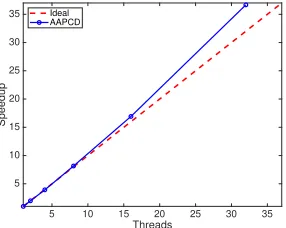
5 10 15 20 25 30 35
Threads
5 10 15 20 25 30 35
Speedup
Ideal AAPCD
Figure 1: Speedup results of AAPCD onrcv1dataset.
The convergence rates in Theorem 7 match the results from (Davis 2016), but they need the independence assumption be-tween blocks and delays. IfT =0 we obtain a synchronous version of the accelerated coordinate descent, and hence The-orem 7 implies the same rates as given in (Li and Lin 2015) for nonconvex functions.
Remark 6. The characterization of the factorb1in Theorems
6 and 7 is noticeable in a particular way that the delays
greater than T1 contribute to this factor. Since β′′ ≤ 0,
it shows that applying negative momentum for high delay
values could efficiently decrease the value ofb1which results
in acceleration.
Remark 7. The KL property ofF is not necessarily
suffi-cient to ensure that the Lyapunov functionGsatisfies the KL
property. However, sinceG−F is semi-algebraic and the
class of semi-algebraic functions is closed under addition, it
shows thatGis semi-algebraic, which implies thatGis a KL
function.
Numerical Results
In this section we test the efficiency of the asynchronous stochastic proximal coordinate descent algorithm with mo-mentum acceleration. We performed binary classifications on the benchmark dataset rcv1. Following the practices in (Gong et al. 2013), we consider the logistic loss function with nonconvex regularization,
g(x)=λ m
∑
j=1
min(|xj|, θ),
for positive momentum and thresholdT1 =0.9τ. All blocks
are of size 1000. We set the stepsize for ASCD withη =0.06. In AASCD we setη=0.09, with momentum valueθ1=0.8.
For DSPG, the stepsize isη =0.03 and mini-batch size is 200. All algorithms are terminated when the number of itera-tions exceeds 100. Note that we use the best tuned parameters for each method which is obtained over a refined grid to at-tain the best performance. Figure 2 shows the convergence of the objective function with respect to CPU time and the number of iterations. Towards the end AAPCD decreases
0 50 100 150
Time(seconds) 10-3
10-2 10-1 100
Training loss - optimum
DSPG ASCD AASCD AAPCD
(a) a
0 20 40 60 80 Iterations 10-4
10-3 10-2
10-1 100
Training loss - optimum
DSPG ASCD AASCD AAPCD
(b) b
Figure 2: Figure(a) is convergence of objective value vs. time; Figure(b) is comparison of the objective function vs. iteration for different algorithms.
rapidly and needs much fewer iterations and less computing time than ASCD and AASCD to reach the same objective function values. This means that our AAPCD algorithm is very efficient and attains the best performance. Moreover AAPCD obtains a much smaller objective value by order of magnitudes compared with other algorithms. For saving space, we leave another experiment for Sigmoid loss in the supplementary materials.
Figure 3 shows AAPCD by only applying nonnegative momentum values which is slower than AAPCD, showing that linear extrapolation using negative momentum β for large delays is significantly useful.
0 50 100 150
Time(seconds) 10-3
10-2 10-1 100
Training loss - optimum
AAPCD AAPCD( >0)
Figure 3: AAPCD versus AAPCD with momentum values β >0.
In summary our experimental results validate that AAPCD can indeed accelerate the convergence in practice.
Conclusion
In this paper, we have studied the stochastic and deterministic asynchronous parallelization of coordinate descent algorithm
with momentum acceleration for efficiently solving noncon-vex nonsmooth problems. We have shown that every limit point is a critical point and proved the convergence rates for deterministic AAPCD with bounded delay. We verified the advantages of our method through numerical experiments.
Overall speaking, these asynchronous proximal algorithms can be highly efficient when being used to solve large scale nonconvex nonsmooth problems. As for future work, an ex-tension of this study might develop the analysis in this paper to inexact proximal methods. We also plan to investigate the asynchronous parallelization of more algorithms for noncon-vex nonsmooth programming for solving more complicated models.
Acknowledgements
This work is partially supported by NSF IIS-1741431 award.
References
Allen-Zhu, Z., and Hazan, E. 2016. Variance reduction for faster non-convex optimization. InInternational Conference
on Machine Learning, 699–707.
Allen-Zhu, Z. 2017. Natasha: Faster non-convex stochas-tic optimization via strongly non-convex parameter. arXiv
preprint arXiv:1702.00763.
Avron, H.; Druinsky, A.; and Gupta, A. 2015. Revis-iting asynchronous linear solvers: Provable convergence rate through randomization. Journal of the ACM (JACM)
62(6):51.
Beck, A., and Teboulle, M. 2009. A fast iterative shrinkage-thresholding algorithm for linear inverse problems. SIAM
journal on imaging sciences2(1):183–202.
Blondel, M.; Seki, K.; and Uehara, K. 2013. Block coor-dinate descent algorithms for large-scale sparse multiclass classification.Machine learning93(1):31–52.
Bolte, J.; Sabach, S.; and Teboulle, M. 2014. Proximal alter-nating linearized minimization or nonconvex and nonsmooth problems. Mathematical Programming146(1-2):459–494. Boţ, R. I.; Csetnek, E. R.; and László, S. C. 2016. An inertial forward–backward algorithm for the minimization of the sum of two nonconvex functions. EURO Journal on
Computational Optimization4(1):3–25.
Davis, D. 2016. The asynchronous palm algorithm for nonsmooth nonconvex problems. arXiv preprint
arXiv:1604.00526.
Dean, J.; Corrado, G.; Monga, R.; Chen, K.; Devin, M.; Mao, M.; Senior, A.; Tucker, P.; Yang, K.; Le, Q. V.; et al. 2012. Large scale distributed deep networks. InAdvances in neural
information processing systems, 1223–1231.
Defazio, A.; Bach, F.; and Lacoste-Julien, S. 2014. Saga: A fast incremental gradient method with support for non-strongly convex composite objectives. InAdvances in neural
information processing systems, 1646–1654.
Ghadimi, S., and Lan, G. 2016. Accelerated gradient meth-ods for nonconvex nonlinear and stochastic programming.
Mathematical Programming156(1-2):59–99.
Gong, P.; Zhang, C.; Lu, Z.; Huang, J.; and Ye, J. 2013. A general iterative shrinkage and thresholding algorithm for non-convex regularized optimization problems. In
Interna-tional Conference on Machine Learning, 37–45.
Gu, B.; Huo, Z.; and Huang, H. 2016. Inexact proximal gra-dient methods for non-convex and non-smooth optimization.
arXiv preprint arXiv:1612.06003.
Hannah, R.; Feng, F.; and Yin, W. 2018. A2bcd: An asyn-chronous accelerated block coordinate descent algorithm with optimal complexity.arXiv preprint arXiv:1803.05578. Leblond, R.; Pedregosa, F.; and Lacoste-Julien, S. 2017. Asaga: Asynchronous parallel saga. InArtificial Intelligence
and Statistics, 46–54.
Li, H., and Lin, Z. 2015. Accelerated proximal gradient methods for nonconvex programming. InAdvances in neural
information processing systems, 379–387.
Li, Q.; Zhou, Y.; Liang, Y.; and Varshney, P. K. 2017. Con-vergence analysis of proximal gradient with momentum for nonconvex optimization. In International Conference on
Machine Learning, 2111–2119.
Lin, Q.; Lu, Z.; and Xiao, L. 2015. An accelerated random-ized proximal coordinate gradient method and its application to regularized empirical risk minimization. SIAM Journal
on Optimization25(4):2244–2273.
Liu, J.; Wright, S. J.; Ré, C.; Bittorf, V.; and Sridhar, S. 2015. An asynchronous parallel stochastic coordinate de-scent algorithm.The Journal of Machine Learning Research
16(1):285–322.
Liu, J.; Chen, J.; and Ye, J. 2009. Large-scale sparse lo-gistic regression. InProceedings of the 15th ACM SIGKDD international conference on Knowledge discovery and data
mining, 547–556. ACM.
Meng, Q.; Chen, W.; Yu, J.; Wang, T.; Ma, Z.; and Liu, T.-Y. 2016. Asynchronous accelerated stochastic gradient descent.
InIJCAI, 1853–1859.
Nesterov, Y. E. 1983. A method for solving the convex programming problem with convergence rate o (1/kˆ 2). In
Dokl. Akad. Nauk SSSR, volume 269, 543–547.
Recht, B.; Re, C.; Wright, S.; and Niu, F. 2011. Hogwild: A lock-free approach to parallelizing stochastic gradient de-scent. InAdvances in neural information processing systems, 693–701.
Reddi, S. J.; Hefny, A.; Sra, S.; Poczos, B.; and Smola, A. J. 2015. On variance reduction in stochastic gradient descent and its asynchronous variants. InAdvances in Neural
Infor-mation Processing Systems, 2647–2655.
Reddi, S. J.; Hefny, A.; Sra, S.; Poczos, B.; and Smola, A. 2016a. Stochastic variance reduction for nonconvex opti-mization. InInternational conference on machine learning, 314–323.
Reddi, S. J.; Sra, S.; Póczos, B.; and Smola, A. J. 2016b. Proximal stochastic methods for nonsmooth nonconvex
finite-sum optimization. InAdvances in Neural Information
Processing Systems, 1145–1153.
Richtárik, P., and Takáč, M. 2014. Iteration complexity of randomized block-coordinate descent methods for mini-mizing a composite function. Mathematical Programming
144(1-2):1–38.
Shalev-Shwartz, S., and Tewari, A. 2011. Stochastic methods for l1-regularized loss minimization. Journal of Machine
Learning Research12(Jun):1865–1892.
Shalev-Shwartz, S., and Zhang, T. 2014. Accelerated proximal stochastic dual coordinate ascent for regularized loss minimization. InInternational Conference on Machine
Learning, 64–72.
Sun, T.; Hannah, R.; and Yin, W. 2017. Asynchronous coor-dinate descent under more realistic assumptions. InAdvances
in Neural Information Processing Systems, 6182–6190.
Xiao, L., and Zhang, T. 2014. A proximal stochastic gradient method with progressive variance reduction. SIAM Journal
on Optimization24(4):2057–2075.
Xu, Y., and Yin, W. 2015. Block stochastic gradient iteration for convex and nonconvex optimization. SIAM Journal on
Optimization25(3):1686–1716.
Yao, Q.; Kwok, J. T.; Gao, F.; Chen, W.; and Liu, T.-Y. 2017. Efficient inexact proximal gradient algorithm for nonconvex problems. In Proceedings of the 26th International Joint
Conference on Artificial Intelligence, 3308–3314. AAAI
Press.