The Thirty-Third AAAI Conference on Artificial Intelligence (AAAI-19)
Zero Shot Learning for Code Education:
Rubric Sampling with Deep Learning Inference
Mike Wu,
1Milan Mosse,
1Noah Goodman,
1,2Chris Piech
11Department of Computer Science, Stanford University, Stanford, CA 94305
2Department of Psychology, Stanford University, Stanford, CA 94305
{wumike,mmosse19,ngoodman,piech}@stanford.edu
Abstract
In modern computer science education, massive open online courses (MOOCs) log thousands of hours of data about how students solve coding challenges. Being so rich in data, these platforms have garnered the interest of the machine learn-ing community, with many new algorithms attemptlearn-ing to au-tonomously provide feedback to help future students learn. But what about those first hundred thousand students? In most educational contexts (i.e. classrooms), assignments do not have enough historical data for supervised learning. In this paper, we introduce a human-in-the-loop “rubric sam-pling” approach to tackle the “zero shot” feedback challenge. We are able to provide autonomous feedback for the first stu-dents working on an introductory programming assignment with accuracy that substantially outperforms data-hungry al-gorithms and approaches human level fidelity. Rubric sam-pling requires minimal teacher effort, can associate feedback with specific parts of a student’s solution and can articulate a student’s misconceptions in the language of the instructor. Deep learning inference enables rubric sampling to further improve as more assignment specific student data is acquired. We demonstrate our results on a novel dataset from Code.org, the world’s largest programming education platform.
Introduction
The need for high quality education at scale poses a diffi-cult challenge. The price of education per student is grow-ing faster than economy-wide costs (Bowen 2012), limitgrow-ing the resources available to support student learning. When also considering the rising need to provide adult retraining, the gap between the demand for education and our ability to provide is especially large. In recent years, massively open online courses (MOOCs) from platforms like Coursera and Code.org have made progress by scaling the delivery of con-tent. However, MOOCs largely ignore an equally important ingredient for learning: high qualityfeedback. The clear so-cietal need, alongside massive amounts of data has led to a machine learning grand challenge: learn how to provide feedback for education at scale, especially in computer sci-ence due to its apparent structure and high demand.
Scaling feedback (a.k.a. “feedback” challenge) has proven to be a hard machine learning problem. Despite
Copyright c⃝2019, Association for the Advancement of Artificial Intelligence (www.aaai.org). All rights reserved.
dozens of projects to combine massive datasets with cutting edge deep learning, current approaches fall short. Three is-sues emerge: (1) for even basic computer science education, homework datasets have statistical distributions with heavy tails similar to natural language; (2) hand labeling feedback is expensive, rendering supervised solutions infeasible; (3) in real world contexts feedback is needed for assignments with small (or zero) historical records of student learning. For the billions of learners around the world, most education and assessments haveat mosthundreds of records. Even if students use Code.org, assignments are constantly changing, making the small-data context perennial. It is a zero-shot so-lution that has potential to deliver enormous social impact.
We build upon a simple insight that enables us to move be-yond the supervised paradigm: When experts give feedback, they are asked to perform the hard task of predicting mis-conception (y) given program (x). When breaking down the cognitive steps that experts go through, they often solve the inference by first thinking generativelyp(x, y). They imag-ine, “if a student were to have a particular set of misconcep-tions, what sorts of programs is he or she likely to produce.” Thinking generatively is much easier: while there are a fi-nite set of decomposable misconceptions, they combine into exponential amounts of unique solutions.
We formalize this intuition into a technique we call “rubric sampling” to elicit samples from an expert prior of the joint distributionp(x, y)and use deep learning for infer-ence p(y|x). With no historical examples, rubric sampling enables feedback with accuracy close to the fidelity of hu-man teachers, outperforming data-intensive state of the art algorithms. We case study this technique on Code.org, an online programming platform that has been used by 610 lion students and has provided a full curriculum to 29 mil-lion students, equivalent to 39% of the US K12 population.
Specific contributions in this paper:
1. We introduce the Zero Shot Feedback Challenge on a dataset from 8 assignments from Code.org along with an evaluation set of 800 labels.
3. We introduce the ability to (i) attribute feedback to spe-cific parts of code, (ii) trace learning over time and (iii) generate synthetic datasets.
The Zero Shot Feedback Challenge
The “Zero-Shot” Feedback Challenge is to infer the miscon-ceptions that led to errors in a student’s answer using zero historical examples of student work and zero expert anno-tations. Though this challenge is difficult, it is a task that humans find straightforward. Experts are especially adept at generalizing: an instructor does not need to see thousands of instances of a misunderstanding in order to understand it.Why is zero-shot so important?Human annotated
exam-ples are surprisingly time consuming to acquire. In 2014, Code.org launched an initiative where hundreds of thou-sands of instructors were crowdsourced to provide feedback to student solutions1. Labeling was hard and undesirable
work and the long tail of unique solutions meant that even after thousands of human hours of teacher work, the annota-tions were only scratching the surface of feedback. The ini-tiative was cancelled after two years and the effort has not been reproduced since. For small classrooms and massive online platforms alike, it is infeasible to acquire the supervi-sion required for contemporary nonlinear methods.
We foresee three main approaches: (1) learn to transfer information from one assignment to another, (2) learn to in-corporate expert knowledge, and (3) form algorithms that can generalize from small amounts of human annotations.
Related Work
Education Feedback If you were to solve an assignment on Code.org today, the hints you would be given are gen-erated from a unit test system combined with static anal-ysis of the students solution. It has been a widely reported social-good objective to improve upon these hints (Price and Barnes 2017) especially since the state of the art is far from ideal (O’Rourke, Ballweber, and Popovi´ı 2014). Achieving this goal has proved to be hard. Previous research on a more basic set of Code.org challenges (the “Hour of Code”) have scratched the surface with respect to providing feedback at scale. Original work found that latent patterns inhow stu-dents solve programming assignments have signal as to how he or she should proceed (Piech et al. 2015c). Applying a neural network improved prediction of feedback (Piech et al. 2015a) but models were (1) too far from human accuracy, (2) weren’t able to explain its predictions and (3) required massive amounts of data. The current state of the art com-bines these ideas and provides some improvements (Wang et al. 2017a). In this paper we propose a method which uses less data, approaches human accuracy and works on more complex Code.org assignments by diverging from the clas-sic supervised framework. Research on feedback for even more complex assignments such as medical education (Gei-gle, Zhai, and Ferguson 2016) and natural language ques-tions (Bulgarov and Nielsen 2018) has also relied on data-hungry supervised learning and perhaps would benefit from a rubric sampling inspired approach.
1
http://www.code.org/hints
Theoretical inspiration for our expert-based generative rubric sampling derives from Brown’s “Repair Theory” which argues that the best way to help students is to un-derstand the generative origins of their mistakes (Brown and VanLehn 1980). Simulating student cognition has been ap-plied to simple arithmetic problems (Koedinger et al. 2015) and recent hard coded models have been very successful in inferring why students make subtraction mistakes (Feld-man et al. 2018). Researchers have argued that such expert models are infeasible for assignments as complex as coding (Paaßen et al. 2017). However, the automated hierarchical decomposition achieved by (Nguyen et al. 2014) inspired us to develop rubric sampling, a simple expert model that works for programming assignments.
Zero Shot Learning There is a growing body of work in zero shot learning from the machine learning community, spawned by poor performance on unseen data.
The simplest approach is to include a human-in-the-loop. While labeling is one way human experts can “teach” a model, it is often not the most efficient. Instead, (Lee et al. 2017) leverages knowledge graphs build by humans to esti-mate a similarity score. Similarly, (Lake, Salakhutdinov, and Tenenbaum 2015) present a probabilistic knowledge graph (i.e. a Bayesian program) for generating symbols that out-perform deep learning on out-of-sample alphabets. In this work, we employ a specific knowledge graph called a gram-mar, which we find to improve generalization.
A more complex approach (without human involvement) focuses on unsupervised algorithms to estimate the data dis-tribution. (Verma et al. 2018; Wang et al. 2017b) train an ad-versarial autoencoder by generatingsyntheticexamples and concurrently fitting a discriminator to classify between syn-thetic and empirical data. (Xian et al. 2018) propose a sim-ilar method for a CNN feature space. In this paper, we gen-eralize this technique to a larger class of (non-differentiable) models: in lieu of a discriminator, we interpolate between synthetic and empirical data via a multimodal autoencoder.
The Code.org Exercises Dataset
Code.orgis an online education platform for teaching
begin-ners fundamental concepts in programming. Students build their solutions in a drag-and-drop interface that pieces to-gether blocks of code. Its growing popularity since 2013 has captured a large audience, having been used by 610 million students worldwide. We investigate a single curriculum con-sisting of 8 exercises from Code.org’s catalog. In this partic-ular unit, students are learning to combine nested for loops with variables, and particularly the use of a for loop counter in calculations. The problems are all presented as drawing geometric shapes in a 2D coordinate space, requiring knowl-edge of angles. For instance, the curriculum begins with the task of drawing an equilateral triangle (see Figure 1).
P1 15,692 / 51,073 P2 50,190 / 48,606 P3 35,545 / 44,819 P4 12,905 / 42,995 P5 27,200 / 42,361 P6 59,693 / 41,198 P7 46,446 / 38,560 P8 59,615 / 36,727
Figure 1: The curricula for learning nested for loops in Code.org. To provide intuition on the vast domain complexity, we show the number of unique solutions (blue) and the number of students (orange) who attempted the problem for each of the 8 exercises.
not have a bounded solution space, students could produce arbitrarily long programs. This implies that, much like natu-ral language, the distribution of student submissions has ex-tremely heavy tails. Figure 2 shows how closely the submis-sions follow a Zipf distribution. To emphasize the difficulty, even after a million students, there is still a 15% chance that a new student generates a solution never seen before.
Head
Body
Tail
Figure 2: The distribution of programs for 8 problems from Code.org follow closely to a Zipf distribution, as shown by the linear relationship between the log probability of a pro-gram and the log of its rank in frequency. 5 to 10 propro-grams dominate while the rest are in the heavy tails.
Evaluation Metric If we only cared about accuracy, we would prioritize the handful of 5 to 10 programs that make up the majority of the dataset. But given the infinite number of possible programs, struggling students who would benefit most from feedback will almost certainly not submit any one of the “most likely” programs. Knowing this, we define our evaluation metrics in terms of the Zipf itself: let thehead(of the Zipf) refer to the top 20 programs ordered by frequency, thetailas any program with a frequency of three or less, and thebodyas everything in between. Figure 2 shows the rough placement of these three splits. When evaluating models, we ignore the head: thesevery commonprograms can be manu-ally labeled. Instead, we will report two F1 scores2: one for
programs in the body and one for the tail.
Human Annotations We collected fine-grained human annotations to over 800uniquesolutions (chosen randomly from P1 and P8) from 7 teaching assistants from the Stan-ford introduction to programming course. We chose to label
2
We choose F1 score over accuracy as the labels are not close to balanced. Thus, accuracy tends to overinflate numbers.
programs from the easiest (P1) and hardest (P8) exercises as they are most different. Intermediate exercises (P2 to P7) share many of same structural features. The annotations are binary labels of 20 misconceptions that cover geometric con-cepts (e.g. doesn’t understand equilateral is 60 degrees) to control flow concepts (e.g. repeats code instead of using a loop). 200 annotations were used to measure inter-rater reli-ability and the remaining 600 were used for evaluation. We refer to this dataset asD. Labeling took 25.9 hours (117 sec-onds per program). At this rate, the entire dataset would take 9987 hours of expert time, over a year of continual work.
Methods
We consider learning tasks given a dataset ofnlabeled ex-amples, where each example (indexed by i) has an input stringxiand a target output vectoryi = [yi,1, ..., yi,l]
com-posed oflindependent binary labels. In this context, we as-sume each string represents a block-based program in Lisp-like notation. Specifically, a program string is a sequence of
Ti tokens, each representing either an operator (functions, for loop, if statements, etc.), an operand (i.e. variable), an open parenthesis “(”, or a close parenthesis “)”. See List-ing 1 for an example program. Formally then, we describe the dataset as:D={xi, yi}ni=1wherexi= [xi,1, ..., xi,Ti].
The goal is to learn a functionyˆi=f(xi)such that we
min-imize the error metric defined above,err(ˆyi, yi). For
super-vised approaches, we splitDinto a training (Dtrain) and test
set (Dtest) via a 80-20 ratio. For unsupervised methods, we
evaluate on the entire setD.
Listing 1: Examplexifrom P1 with 51 tokens. The tokens
ProgramandWhenRunserve the role of a start-of-sentence
tokens. A model will receive each token in order. ( P r o g r a m ( WhenRun ) ( Move ( F o r w a r d
) ( V a l u e ( Number ( 50 ) ) ) ) ( R e p e a t ( V a l u e ( Number ( 3 ) ) ) ( Body ( T u r n ( L e f t ) ( V a l u e ( Number ( 120 ) ) ) ) ) ) )
Baselines
Majority Label As a sanity check, we can naively make predictions by voting for the majority label fromDtrain.
Predicting from Output The ubiquitous way to provide feedback is via unit tests: analyze the output of executing
when run TurnTurn Left {integer}Right
Terminal Nodes
done
when run Turn Left 3 1000
Move forward
Move forward repeat until
do repeat for do
{string} …
…
For loop: wrong end For loop: wrong end
For loop: correct
For loop: no loop
Start Token
Move: wrong op
Move: wrong op
Turn: no turn
Turn: Correct
For loop: Correct
Move: wrong multiple
For loop: correct Program (start token)
Move: wrong op
Move: wrong multiple
Non-Terminal Nodes
i) primitives ii) token emission iii) merge tokens
terminal relation: emission of code
synthetic program: example output sampled
from grammar
synthetic feedback: we get semantic tags as
part of the generation non-terminal relation: mimic student thinking
repeat for do
when run Turn Left
Move forward 1000 repeat for 3 do
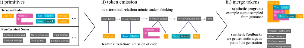
Figure 3:Probabilistic grammar (PCFG) for synthetic block-based programs.To generate a synthetic example, we sequentially choose a set of non-terminal nodes, each of which will emit a set of terminal nodes. The composition of these terminal nodes make up a program whereas the composition of non-terminal nodes make up the labels/feedback. The emission and transition probabilities are specified by a human designer (or learned via evolutionary strategies).
of output vectorsoi = (oi,1, oi,2, ...)representing
coordi-nates in 2D space where a line has been drawn. We train a recurrent neural network (RNN) to predictyi fromoi.
Un-fortunately, this model requiresxito compile.
Feedforward Neural Network To circumvent compila-tion, one can tackle the more difficult problem of predict-ing feedback from raw program strpredict-ings (Piech et al. 2015b). We train al-dimensional classifier composed of a RNN over tokens by minimizing the binary cross entropy between pre-dictionsyˆiand ground truthyivectors.
min
l ∑
j=1
[−(yi,jlog ˆyi,j) + (1−yi,j) log(1−yˆi,j)] (1)
The model architecture borrows the sentence encoder (with-out any stochastic layers) from (Bowman et al. 2015) and concatenates a 3-layer perceptron with a softmax overl out-put dimensions. As we will reuse these architectures for other models, we refer to deterministic encoder as the
pro-gram networkand the latter MLP as thefeedback network.
Trajectory Prediction No model so far uses the fact that each student submits many programs before either stopping or reaching the correct solution. In fact, the current SOTA (Wang et al. 2017a) is to associate atrajectoryofkprograms
(x1, x2, ..., xk)with the label yi corresponding to the last
program,xk. Then, for each programxi, we train an
embed-dingei=f(z|xi), wheref is the program network. This
re-sults in a sequence of embeddings(e1, e2, ..., ek)for a single
trajectory. We concurrently train asecondRNN to compress the sequence to a single vector zi = RNN(e1, e2, ..., ek).
This is then provided as input to the feedback network. The hope is that structure induced by a trajectory implicitly pro-vides labels that strengthen learning.
Deep Generative Model Finally, we present a new base-line that is promising in the context of limited data. If we consider programs and feedback as two modalities, one ap-proach is to capture the joint distributionp(xi, yi). Doing
so, we can make predictions by sampling from the con-ditional having seen the program: yˆi ∼ p(yi|xi). To do
this, we train a multimodal variational autoencoder, MVAE (Wu and Goodman 2018) with two channels. Succinctly,
this generative model uses a product-of-experts inference network where the joint distribution factorizes into a prod-uct of distributions defined by two modalities:q(z|x, y) =
q(z|x)q(z|y) where xand y are two observed modalities andzis a latent variable. We optimize the multimodal ev-idence lower bound (Wu and Goodman 2018; Vedantam et al. 2017), which is a sum of three lower bounds:
E qφh(z|x,y)
[ ∑
h∈{x,y}
λhlogpθh(h|z)]−βKL[qφh(z|x, y), p(z)]
+ E
qφx(z|x)
[logpθx(x|z)]−βKL[qφx(z|x), p(z)]
+ E
qφy(z|y)
[logpθyy|z)]−βKL[qφy(z|y), p(z)] (2)
To parameterizeqφx andpθx, we use architectures from
(Bowman et al. 2015). For qφy and pθy, we use 3-layer
MLPs3. To the best of our knowledge, this is the first
appli-cation of a deep generative model to the feedback challenge.
Rubric Sampling
So far the models have been severely constrained by the number of labels. If we had a more efficient labeling strat-egy, we could better train these deep models to their full po-tential. For instance, imagine instead of focusing on individ-ual programs, we ask experts to describe a student’s thought process, enumerating strategies to get to a right or wrong an-swer. Given a detailed enough description, we can use it to label indefinitely. Granted, these labels will be noisy but the quantity should make up for any uncertainty. In fact, we can formalize such a “description” as acontext-free grammar.
A context-free grammar (CFG) is composed of a set of acyclic production rules describing a space of output strings. As its name suggests, each rule is applied regardless of context (meaning no conditional arguments). Formally, a production rule is made up of non-terminal andterminal
symbols. Non-terminal symbols are hidden and either pro-duce another non-terminal symbol or a terminal one. Ter-minal symbols are made up of tokens that appear in the fi-nal output string. For instance, consider the following CFG: S →AA;A→α;A→β. S and A are non-terminal sym-bols whereasαandβare terminal. It is easy to see that this
3
qφx(z|x)is composed of the program network and a stochastic
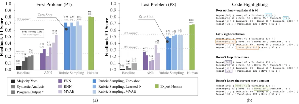
Figure 4: (a) The F1 scores for P1 and P8. We plot two bars for each model representing the F1 score on the body (left) and on the tail (right). Rubric sampling models perform far better than baselines and grow close to human-level. The “Zero Shot” marking refers to rubric sampling without fine-tuning. (b) Highlighting sub-programs conditioned on 4 feedback labels. The MVAE contains a modality for highlighting masks generated using the rubric. Imagine programming education where sections of a student’s code can be highlighted along with helpful diagnostics.
CFG can only generate one of{αβ, βα, αα, ββ}. A
proba-bilisticcontext-free grammar (PCFG) is a CFG
parameter-ized by a vectorθwhere each production rule has a proba-bilityθiattached. For example, we can make our CFG from
above probabilistic: S −−→1.0 AA;A −−→0.9 α;A −−→0.1 β. Now, the space of possible outputs has not changed but for in-stance,αβwill be more probable thanβα.
For the feedback challenge, the non-terminal symbols are labels,yi and the terminal symbols are programs, xi. For
example, a possible production rule might be:
Correctly identified 45 degree angle−−→1.0 T urn(45)
With a PCFG, we can generate an infinite amount of syn-thetically labeled programs,Dsyn = {xi, yi}, and useDsyn
to train data-hungry models. We refer to this asrubric
sam-pling. In practice, we sample a million synthetic examples.
When training supervised networks, we only include unique examples to avoid prioritizing programs in the Zipf head.
Creating rubrics is surprisingly easy. For a novice (under-graduate) and an expert (professor), making a PCFG took 19.4 minutes. To make the process even easier, we devel-oped a simple meta language for representing a grammar.4
Further Learning from Unlabeled Programs
As students use the platform, unlabeled submissions accu-mulate over time. We refer to the dataset asDunlabeled.
Evolutionary Strategies We can use unlabeled data in rubric sampling to automatically learn θ. This means alle-viating some of the burden for a human-in-the-loop, since choosingθis often more difficult than designing the gram-mar itself. Intuitively, it is easier to reason about what mis-takes a student can make than how often a student will make
4
A Pytorch implementation, rubric grammars, along with data can be found at https://github.com/mhw32/rubric-sampling-public.
each mistake. But since a PCFG is discrete, we cannot dif-ferentiate. However, we can hope to approximate local gra-dients by sampling θ values within some ϵ-neighborhood and computing finite differences along these random direc-tions (Salimans et al. 2017). If we repeatedly take a linear combination of the “best” samples as measured by afitness
function, then over many iterations, we expect the PCFG to improve. The challenge is in picking the fitness function.
A good choice is to pickθwhose generated distribution,
Dsyn is “closest” to Dunlabeled5. As both are Zipf-ian, we
can properly measure “closeness” using a rank order met-ric (Havlin 1995), as rank is independent of frequency.
Rubric Sampling with MVAE Another way to service unlabeled data is to train with it: one of the features of the MVAE is that it can handle missing modalities. We can fit the MVAE withtwodata sources:DsynandDunlabeled.
In the case of missing labels, Equation 2 decomposes into the (unimodal) ELBO (Wu and Goodman 2018):
E qφx(z|x)
[logpθx(x|z)]−βKL[qφx(z|x), p(z)] (3)
Thus, the MVAE is shown both a synthetic minibatch,
(xi, yi) ∼ Dsyn, which is used to compute the
multi-modal elbo, and an unlabeled minibatch,(xi) ∼Dunlabeled,
which computes Equation 3. We can jointly optimize the two losses by summing the gradients prior to taking an optimiza-tion step. Intuitively, this interpolates betweenDunlabeledand
Dsyn, no longer completely relying on the PCFG. One can
also interpret this as a soft-version of structure learning since usingDunlabeledis somewhat akin to “editing” the PCFG.
5
D
unlabeledD
generatedlog-zipf exp-zipf
MVAE
D
~
unlabeledD
~
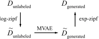
generatedFigure 5: log-Zipf transformation. Applying a log to fre-quencies ofxi∼Dis like “tempering”. This helps mitigate
the effect of a few elements dominating the distribution.
Log-Zipf Transformation Capturing a Zipf is hard for a generative model since it is very easy to memorize the top 5 programs and very hard to capture the tail. To make it easier, we apply alogtransformation,6e.g. if a program appears 10 times inD, it only appears once in the transformed dataset,
˜
D. Then, when generating with the MVAE, we invert the log by exponentiating the frequency of each unique program (exp-Zipf). Intuitively, log-Zipf is similar to “tempering” a distribution as it reduces any extreme peaks and troughs.
Results
Recreation of Human Labels
Figure 4 reports a set of F1 scores, including human-level performance estimated from annotations. Each model is given two bar plots, one for programs in the body (left) and one in the tail (right). First, we see that baselines have lower F1 scores compared to models that take advantage of synthetic data. That being said, the new baseline MVAE we introduced already performs far better than the previous SOTA. In P1, using rubric sampling increases the F1 score by 0.31 in the body and 0.13 in the tail (we find similar gains in P8). These promising results imply that the grammar in-deed is effective. We also find that combining the MVAE with rubric sampling boosts the F1 by an additional 0.2, reaching 94% accuracy in P1 and 95% in P8. With these scores, we are reasonably confident that for a new student, despite the likelihood that he/she will submit a never-before-seen program, we will provide good feedback.
To put these results in terms of impact, Table 1 estimates the number of correct feedback we could have given to stu-dents in P1 to P8 based on projections from the annotated set. Over the full curriculum, our best model would have provided the correct feedback to an expected 126,000 addi-tional programs compared to what Code.org currently uses, potentially helping thousands more students.
Tracing Knowledge Across Curricula
If we had a scalable way to provide feedback, what impact could we make to code education? We can begin to mea-sure this impact using the full Code.org curriculum. Having demonstrated good performance on P1 and P8, we can confi-dently apply rubric sampling to P2 through P7. This is quite powerful as it allows us to estimate student understanding
6
We preserve examples that appear only once inDto D˜ i.e.
˜
x= min(log(x),1)wherex∈Dandx˜∈D˜.
Model
Amount of Correct Feedback Predicting from output 1,483,157 (86.0%) Rubric sampling with MVAE 1,610,020(93.7%) Expert human 1,658,162 (96.2%)
Table 1: Amount of correct feedback over the curriculum.
We ignore programs in the head of the Zipf as those can be manually labeled. With the best model, we could have provided 126,000 additional points of feedback.
over a curricula. Critically, we can gauge the performance of both individual students and the student body as a whole. These sort of queries are valuable to teachers to be able to (1) measure a student’s progress scalably and (2) judge how useful assignments and lessons have been.
In Figure 6, we analyze the average student’s level of understanding over the 8 problems for two main concepts: loops and geometry (e.g. shapes, angles, movement). For each submission in a student’s trajectory, we classify it as having either 1) no errors, 2) more loop errors, or 3) more geometry errors7. The figure shows the distribution of
stu-dents in each of the three categories from the first 10 sub-missions. From looking at behavior within a problem and between problems, we can make the following inferences:
1. Most students are successfully completing each prob-lem.In other words, the blue area is increasing over time. Equivalently, the number of students still struggling by the 10th submission approaches a small number.
2. The difficulty of problems is not uniform.P6 is much more difficult than the others as the fraction of students with correct solutions is roughly constant. In contrast, P1, P4, and P5 are easier, where students quickly cease to make mistakes. As a teacher, one could use this informa-tion to improve the educainforma-tional content and better hone in on areas where more students struggle.
3. Students are learning geometry better than looping. The rate that the pink area approaches zero is consistently faster than that of the orange area. By P8, students are barely struggling with geometry but a fair proportion still find looping difficult. As the curriculum was intended to teach nested looping, one interpretation is that the draw-ing aspect was somewhat distractdraw-ing.
Fine-grain Feedback: Code Highlighting
With most online programming education, the form of feed-back is limited to pop-up tips or compiler messages. But, with generative models we can provide more fine-grain feed-back throughhighlightingsubsets of the program responsi-ble for the model predicting each feedback label.
7We do so by comparing the summed predicted probabilities
for all labels related to loops,yˆi,loop=∑j∈loopyˆi,j and labels
re-lated to geometry,yˆi,geom =∑j∈geomyˆi,j. If bothyˆi,loop <1and ˆ
yi,geom <1, then we classify this program as “no errors”.
P1 P2 P3 P4 P5 P6 P7 P8
P
er
ce
nt
of
S
tude
nt
s
P
er
ce
nt
C
or
re
ct
0.0 100.0
0.0 100.0
Submission Number
0 5 10 0 5 10 0 5 10 0 5 10 0 5 10 0 5 10 0 5 10 0 5 10 0 5 10 0 5 10 0 5 10 0 5 10 0 5 10 0 5 10 0 5 10 0 5 10
Submission Number
More Geometry Errors
More Loop Errors
No Errors
Geometry Feedback
Loop Feedback
Figure 6:Student understanding of loops and geometry across curricula: (top row) We plot the percentage of students who are either doing perfect (cyan), struggling more with looping concepts (orange), or struggling more with geometry concepts (pink). In general the percentage of students with no errors increases over time as more students finish the problem. Additionally, we can extrapolate that students are more effectively learning geometry than looping, as the area covered by pink decreases faster and more consistently than the area covered by orange. We can also see that P6 is somewhat of an outlier, being much more difficult for students than any other problem. (bottom row) In addition to aggregate statistics, we can also track learning for individual students. We can infer that this particular student tries several attempts with P6 before dropping out.
First, if we consider a PCFG, the task of highlighting a programxi is equivalent to finding the most likely parsing
in a probabilistic tree that would generate xi. In practice,
we use the A* algorithm for fast Viterbi parsing (Klein and Manning 2003). Given the most likely parsing, we can fol-low the trajectory from root to leaf and record which sub-programs are generated by non-terminal nodes. This has one major limitation: only programs within the support of the PCFG can be highlighted. To bypass this, we can curate a synthetic dataset with each program having a segmenta-tion mask denoting which tokens to highlight. If we treat the mask as an additional modality, we can then learn the joint distribution over programs, labels, and masks. See (Wu and Goodman 2018) for details in defining a VAE with three modalities. In Figure 4b, we randomly sample 4 programs and show segmentation masks. The running time to compute a mask is negligible, meaning that this can be used for pro-viding on-the-fly feedback to students. Moreover, highlight-ing provides a notion of interpretability (which is extremely important if we are working with students), much like Grad-Cam (Selvaraju et al. 2017) did for computer vision.
Clustering Students by Level of Understanding
With any latent generative model, the rich latent space pro-vides a vector representation for unstructured data. Using the MVAE, we first samplezi ∼q(zi|xi)for allxi∈Dtest;
we then train use t-SNE (Maaten and Hinton 2008) to re-duce to two dimensions. In Figure 7b and c, we color each embedded program fromDsynby whether the true label is
positive or negative. We find that the space is partitioned to group programs with similar feedback together. In Figure 7a, we see thatDunlabeledis also organized into disjoint clusters.
This implies that even with no data about a new student we can draw inferences from their neighbors in latent space.
Positive Negative Unlabeled
(a)Dunlabeled (b)Dsyn: Turn/Move (c)Dsyn: No Repeat
Figure 7:Clustering students.Using the inference network in the MVAE, we can embed a program in 2D. InDunlabeled
(a), we see a handful of distinct clusters. In Dsyn(b,c), we
find meaningful clusters that are segmented by labels.
Discussion
We get closer to human level performance than previous SOTA. Any of the rubric sampling models beat the SOTA by at least 0.46 in P1 and 0.24 in P8, nearly tripling the F1 score in P1 and doubling in P8. In both exercises, our best model is just under 95% accuracy, which is encouraging for this to be implemented in the real world.
We can effectively track student growth over time. With a high performing model, we can analyze students over time. For Code.org, we were able to (1) gauge what indi-vidual students struggle with, (2) gauge what a collective of students struggle with, (3) identify the effectiveness of a curriculum, and (4) identify the difficulty of problems.
are much higher than baselines (0.29±,0.03). Furthermore, we measured that it took a group of teaching assistants 24.9 hours to label 800 unique programs. In comparison, it took a novice an average of 19.4 minutes to make a rubric.
We provide feedback to programs that do not compile. Rubic sampling and MVAE make no assumptions on pro-gram behavior, working out-of-the-box from the 1st student.
We do not need to handpickθwhen designing a rubric. In Figure 1, the PCFG uses hand-picked θ. However, one can argue that it is difficult to know how often students make mistakes and yet, the choice ofθis important: performance drops if we randomly choose. For example, in P1, using hand-pickedθhas a0.26±0.002increase over randomθin F1-score. In the absence of an expert, we can use evolution-ary strategies to find a good minima starting from a random initialization. Over 3 runs, we found that learningθreduces the difference to0.007±0.005in P1, even beating expert parameters by0.005±0.009in P8. With a large dataset, we only have to define the structure, not the probabilities.
The log-Zipf transform ensures that learning does not collapse to memorizing the most frequent programs. If we were to use the raw statistics of the student data, the MVAE would minimize loss by memorizing the most fre-quent programs. As evidence of this, when sampling from its generative model, we found that the MVAE only gener-ated programs in the top 25 programs by frequency (even with 1 million samples). We propose the log-Zipf transfor-mation as a general tool for parameter learning with Zipf-distributed data. Critically, the transform downweights the head and upweights the tail in an invertible fashion.
The MVAE interpolates between synthetic and empirical data. Unlike the PCFG, we can train the MVAE with mul-tiple data sources. Effectively, the programs we show to the model is drawn from an interpolation between the synthetic distribution defined by rubric sampling and the true (unla-beled) data distribution. Intuitively, the increase in perfor-mance from the MVAE can be attributed to better capturing the true density of student programs (see Figure 9).
We can generate and open-source a large dataset of stu-dent programs. Datasets with student data are difficult to release to the open community. But large public datasets have been a dominant force in pushing the boundaries of re-search. Luckily, with generative models, we can curate our own “Imagenet” for education. But, we want to ensure that our dataset matchesD in distribution. Intuitively, it is im-possible that a PCFG can capture D since that would re-quire production rules that span the entire tail of the Zipf. In fact, as shown in Figure 8, the PCFG is not that faithful. One remedy is to use the MVAE trained withDunlabeledas that is
interpolating between distributions. Figure 8, confirms that the MVAE matches the shape ofDmuch better.
0 5 10
log Rank
12 10 8 6 4 2
log Probability
Generated Empirical
(a) P1 (PCFG)
0 5 10
log Rank
12 10 8 6 4 2
log Probability
Generated Empirical
(b) P1 (MVAE)
Figure 8: We compareDM V AE
syn andDRubricsyn toDunlabeled.
Programs from the MVAE coverDunlabeledmuch better than
relying on synthetic data alone (PCFG).
Limitations and Future Work
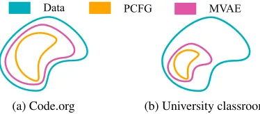
The effectiveness of rubric sampling is largely determined by the complexity of the programming task. Although a block-based language like in Code.org already has an infi-nite number of possible programs, the set of probable stu-dent programs is much smaller than in a typical university level coding assignment. An important distinction is the in-troduction of variable and function names. As suggested by Figure 9, the version of rubric sampling used in this paper may have difficulty scaling to harder problems. As PCFGs are context-free, making a sufficiently expressive grammar for complex problems requires extremely large graphs with repetitive subgraphs. Future work could look to generalizing rubric sampling to arbitrary graphs with conditional branch-ing, or investigate structural learning to improve graphs to cover more of the empirical data.
Data PCFG MVAE
(a) Code.org (b) University classroom
Figure 9: The space of likely student programs in a block-based language can be covered by a PCFG. But in a higher-order language like Python, the space is much larger.
Conclusion
We introduce the zero shot feedback challenge. On a widely used platform, we show rubric sampling to far surpass the SOTA. We combine this with a generative model to clus-ter students, highlight code, and incorporate historical data. This approach can scale feedback for real world use.
Acknowledgments
References
Bowen, W. G. 2012. The cost disease in higher education: is technology the answer? The Tanner Lectures Stanford
University.
Bowman, S. R.; Vilnis, L.; Vinyals, O.; Dai, A. M.; Jozefow-icz, R.; and Bengio, S. 2015. Generating sentences from a continuous space. arXiv preprint arXiv:1511.06349. Brown, J. S., and VanLehn, K. 1980. Repair theory: A gen-erative theory of bugs in procedural skills.Cognitive science
4(4):379–426.
Bulgarov, F. A., and Nielsen, R. 2018. Proposition en-tailment in educational applications using deep neural net-works. InAAAI.
Feldman, M. Q.; Cho, J. Y.; Ong, M.; Gulwani, S.; Popovi´c, Z.; and Andersen, E. 2018. Automatic diagnosis of students’ misconceptions in k-8 mathematics. InProceedings of the 2018 CHI Conference on Human Factors in Computing Sys-tems, 264. ACM.
Geigle, C.; Zhai, C.; and Ferguson, D. C. 2016. An ex-ploration of automated grading of complex assignments. In
Proceedings of the Third (2016) ACM Conference on
Learn-ing@ Scale, 351–360. ACM.
Havlin, S. 1995. The distance between zipf plots. Physica
A: Statistical Mechanics and its Applications216(1-2):148–
150.
Klein, D., and Manning, C. D. 2003. A parsing: fast exact viterbi parse selection. InProceedings of the 2003 Conference of the North American Chapter of the Associ-ation for ComputAssoci-ational Linguistics on Human Language
Technology-Volume 1, 40–47. Association for
Computa-tional Linguistics.
Koedinger, K. R.; Matsuda, N.; MacLellan, C. J.; and McLaughlin, E. A. 2015. Methods for evaluating simulated learners: Examples from simstudent. InAIED Workshops. Lake, B. M.; Salakhutdinov, R.; and Tenenbaum, J. B. 2015. Human-level concept learning through probabilistic pro-gram induction.Science350(6266):1332–1338.
Lee, C.-W.; Fang, W.; Yeh, C.-K.; and Wang, Y.-C. F. 2017. Multi-label zero-shot learning with structured knowledge graphs.arXiv preprint arXiv:1711.06526.
Maaten, L. v. d., and Hinton, G. 2008. Visualizing data using t-sne. Journal of machine learning research9(Nov):2579– 2605.
Nguyen, A.; Piech, C.; Huang, J.; and Guibas, L. 2014. Codewebs: scalable homework search for massive open on-line programming courses. InProceedings of the 23rd
inter-national conference on World wide web, 491–502. ACM.
O’Rourke, E.; Ballweber, C.; and Popovi´ı, Z. 2014. Hint systems may negatively impact performance in educational games. In Proceedings of the first ACM conference on
Learning@ scale conference, 51–60. ACM.
Paaßen, B.; Hammer, B.; Price, T. W.; Barnes, T.; Gross, S.; and Pinkwart, N. 2017. The continuous hint factory-providing hints in vast and sparsely populated edit distance spaces.arXiv preprint arXiv:1708.06564.
Piech, C.; Huang, J.; Nguyen, A.; Phulsuksombati, M.; Sa-hami, M.; and Guibas, L. 2015a. Learning program embed-dings to propagate feedback on student code. InProceedings of the 32nd International Conference on Machine Learning.
Piech, C.; Huang, J.; Nguyen, A.; Phulsuksombati, M.; Sa-hami, M.; and Guibas, L. 2015b. Learning program embed-dings to propagate feedback on student code.arXiv preprint
arXiv:1505.05969.
Piech, C.; Sahami, M.; Huang, J.; and Guibas, L. 2015c. Au-tonomously generating hints by inferring problem solving policies. InProceedings of the Second (2015) ACM
Confer-ence on Learning@ Scale, 195–204. ACM.
Price, T. W., and Barnes, T. 2017. Position paper: Block-based programming should offer intelligent support for learners. InBlocks and Beyond Workshop (B&B), 2017 IEEE, 65–68. IEEE.
Salimans, T.; Ho, J.; Chen, X.; Sidor, S.; and Sutskever, I. 2017. Evolution strategies as a scalable alternative to rein-forcement learning. arXiv preprint arXiv:1703.03864. Selvaraju, R. R.; Cogswell, M.; Das, A.; Vedantam, R.; Parikh, D.; and Batra, D. 2017. Grad-cam: Visual expla-nations from deep networks via gradient-based localization. InICCV, 618–626.
Vedantam, R.; Fischer, I.; Huang, J.; and Murphy, K. 2017. Generative models of visually grounded imagination. arXiv
preprint arXiv:1705.10762.
Verma, V. K.; Arora, G.; Mishra, A.; and Rai, P. 2018. Gen-eralized zero-shot learning via synthesized examples. InThe IEEE Conference on Computer Vision and Pattern
Recogni-tion (CVPR).
Wang, L.; Sy, A.; Liu, L.; and Piech, C. 2017a. Learn-ing to represent student knowledge on programmLearn-ing exer-cises using deep learning. InProceedings of the 10th Inter-national Conference on Educational Data Mining; Wuhan,
China, 324–329.
Wang, W.; Pu, Y.; Verma, V. K.; Fan, K.; Zhang, Y.; Chen, C.; Rai, P.; and Carin, L. 2017b. Zero-shot learning via class-conditioned deep generative models. arXiv preprint
arXiv:1711.05820.
Wu, M., and Goodman, N. 2018. Multimodal genera-tive models for scalable weakly-supervised learning. arXiv
preprint arXiv:1802.05335.
Xian, Y.; Lorenz, T.; Schiele, B.; and Akata, Z. 2018. Fea-ture generating networks for zero-shot learning. In Proceed-ings of the IEEE conference on computer vision and pattern