GPS TEC and ITEC from digisonde data compared with NEQUICK model

Radio Science

GPS TEC and ITEC from digisonde data compared with

NEQUICK model

J.-C. Jodogne1, H. Nebdi1, and R. Warnant1*

1_{Institut Royal M´et´eorologique, 3 Avenue Circulaire, B-1180 Bruxelles, Belgium} *_{Royal Observatory of Belgium}

Abstract. At the Dourbes station, a digisonde 256 is

co-located with a Turbo Rogue GPS receiver. Real time process-ing of the digisonde data gives the electron density profile and the ITEC value (SAO file) for each sounding. The GPS receiver produces data that are treated at the Royal Obser-vatory in order to extract a vertical TEC. Running the well-known NeQuick ionospheric model allows to compute verti-cal TEC values. Comparisons of the results obtained in 1996 and 2001 by these different approaches are shown.

1 Introduction

The use of empirical models for the Total Electron Content (TEC) appears to increase in different applications. We ben-efit of the co-location of two systems able to provide TEC estimations to compare with such a model.

NeQuick model is a one adopted by the COST 251 Action and updated during the succeeding COST 271 Action till now (Leitinger et al., 2002). To be short, the CCIR coefficients are used for foF2 and we run the software program with the monthly averaged solar flux for each hour at the Dourbes lo-cation. The profilers for E-, F1- and F2-regions are Epstein functions with different parameters for bottom and top parts. The topside ionosphere is simply a semi-Epstein layer. One of the features of the NeQuick model is to compute the elec-tron content between any starting point (lat, long and height) and ending point in straight line. We limit ourselves to ver-tical direction. Two graphs for respectively 2001 (high solar activity) and 1996 (low solar activity) displayed at Fig. 1 give an idea of the model behaviour.

A Turbo Rogue receiver was installed at the top of the main building of the Dourbes station for derivation of GPS TEC values (Warnant and Jodogne, 1998). We remove all data from GPS satellite whose elevation is less than 88.5◦_.

Correspondence to: J.-C. Jodogne ([email protected])

At the Dourbes station a digisonde 256 with the Artist soft-ware produces hourly ionograms. The SAO output file gives the usual characteristics and an ITEC (Ionospheric TEC) up to infinity (Huang and Reinisch, 2001). It is such a value automatically produced that was used for this work.

2 NeQuick compared with GPS TEC

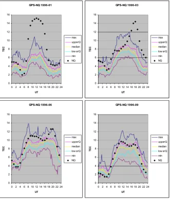
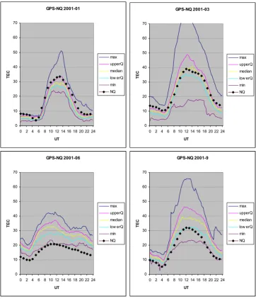
In order to see the data compared with the model we choose several months. GPS TEC was produced each quarters of the hour. We compute the median, the lower and upper quartiles, the maximum and the minimum for each quarter of hour of the month. The graphs present these values. We show the hourly NeQuick values as diamonds on the graphs. Typi-cal season’s months are displayed (January, March, June and September) for the years 1996 and 2001 (Figs. 2 and 3). To easily see the contrast between the two years we put four graphs on one panel.

When the solar activity was low the model gives higher values except for September 1996. For high solar activity values are quite good for January and especially for March but too small during June and September 2001.

3 NeQuick compared with Ionospheric Total Electron

Contents

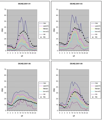
As for the GPS data, we compute the same statistical param-eters for the year 2001. However GPS TEC were produced each quarter of hour but we record hourly ionograms only. Again we show NeQuick values as diamonds on the graphs (Fig. 4).

1

5

9

13

17

21 ₁ 3 5 7 9 11

0 10 20 30 40 50 60 70 TEC UT Month NQ 1996 1 2 3 4 5 6 7 8 9 10 11 12 1 5 9 13 17

21 ₁ 3 5 7 9 11

0 10 20 30 40 50 60 70 TEC UT Month NQ 2001 1 2 3 4 5 6 7 8 9 10 11 12

Fig. 1. TEC values up to 20 000 km from the NeQuick model for 1996 and 2001.

GPS-NQ 1996-01 0 2 4 6 8 10 12 14 16

0 2 4 6 8 10 12 14 16 18 20 22 24

UT TEC max upperQ median low erQ min NQ GPS-NQ 1996-03 0 2 4 6 8 10 12 14 16

0 2 4 6 8 10 12 14 16 18 20 22 24

UT TEC max upperQ median low erQ min NQ GPS-NQ 1996-06 0 2 4 6 8 10 12 14 16

0 2 4 6 8 10 12 14 16 18 20 22 24

UT TEC max upperQ median low erQ min NQ GPS-NQ 1996-09 0 2 4 6 8 10 12 14 16

0 2 4 6 8 10 12 14 16 18 20 22 24

UT TEC max upperQ median low erQ min NQ

GPS-NQ 2001-01

0 10 20 30 40 50 60 70

0 2 4 6 8 10 12 14 16 18 20 22 24

UT

TEC

max upperQ median low erQ min NQ

GPS-NQ 2001-03

0 10 20 30 40 50 60 70

0 2 4 6 8 10 12 14 16 18 20 22 24

UT

TEC

max upperQ median low erQ min NQ

GPS-NQ 2001-06

0 10 20 30 40 50 60 70

0 2 4 6 8 10 12 14 16 18 20 22 24

UT

TEC

max upperQ median low erQ min NQ

GPS-NQ 2001-9

0 10 20 30 40 50 60 70

0 2 4 6 8 10 12 14 16 18 20 22 24

UT

TEC

max upperQ median low erQ min NQ

Fig. 3. Same as Fig. 2 but for year 2001.

In March 2001 we run the digisonde each 30 min. When these data are taken into account we get the graph of Fig. 5. The influence of waves in the ionosphere appears clearly. For some hours, the upper quartiles, medians and lower quartiles have nearly the same values despite the wavy structure (2:00, 3:00, 8:30, 10:30, 12:30, 13:30, 19:30, 20:30, 22:30). For GPS TEC during this month, the difference between the up-per quartile and the lower quartile is small and the model fits quite well the data.

4 Ionospheric Total Electron Contents compared with GPS TEC

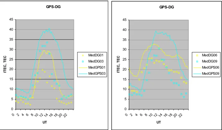
We display the medians for GPS as curves and for digisonde as points (Fig. 6). The shapes of both estimations are quite similar. As well known the GPS values are always larger than those from the digisonde.

5 Conclusions

As TEC estimations from GPS used in this work are means from about 30 samples during 15 min, it is understandable that the scatter of the GPS data is lesser. The night’s data of the two experimental systems seems to be closer (except for June) to the model’s values than those of the day. During daytime the discrepancies can reach more than 50% (January 1996) for GPS.

DG-NQ 2001-01

0 10 20 30 40 50 60 70

0 2 4 6 8 10 12 14 16 18 20 22

UT

ITEC

max upperQ Median low erQ min NQ

DG-NQ 2001-03

0 10 20 30 40 50 60 70

0 2 4 6 8 10 12 14 16 18 20 22

UT

ITEC

max upperQ Median low erQ min NQ

DG-NQ 2001-06

0 10 20 30 40 50 60 70

0 2 4 6 8 10 12 14 16 18 20 22

UT

ITEC

max upperQ Median low erQ min NQ

DG-NQ 2001-09

0 10 20 30 40 50 60 70

0 2 4 6 8 10 12 14 16 18 20 22

UT

ITEC

max upperQ Median low erQ min NQ

Fig. 4. Same as Fig. 3 but ITEC values from SAO files of the digisonde.

DG-NQ 2001-3+

0 10 20 30 40 50 60 70

0 2 4 6 8 10 12 14 16 18 20 22 24

UT

ITEC

max upperQ median lowerQ min NQ

GPS-DG

0 5 10 15 20 25 30 35 40 45

0 2 4 6 8 10 12 14 16 18 20 22 UT

ITEC

, TEC

MedDG01 MedDG03 MedGPS01 MedGPS03

GPS-DG

0 5 10 15 20 25 30 35 40 45

0 2 4 6 8 10 12 14 16 18 20 22 UT

ITEC

, TEC

MedDG06 MedDG09 MedGPS06 MedGPS09

Fig. 6. Medians for digisonde ITEC (points) and GPS TEC (curves) during January and March (left panel) or June and September (right panel).

References

Huang, X. and Reinisch, B. W.: Vertical electron content from iono-grams in real time, Radio Science, 36, 2, 335–342, 2001. Leitinger, R., Radicella, S., and Nava, B.: Electron density models

for assessment studies – new developments, Acta Geodet. Geo-phys. Hung. 37, 183–193, 2002.