The Thirty-Third AAAI Conference on Artificial Intelligence (AAAI-19)
Learning Phenotypes and Dynamic Patient Representations via RNN Regularized
Collective Non-Negative Tensor Factorization
Kejing Yin,
1Dong Qian,
1William K. Cheung,
1Benjamin C. M. Fung,
2Jonathan Poon
31Department of Computer Science, Hong Kong Baptist University, Hong Kong SAR, China 2School of Information Studies, McGill University, Montreal, Canada
3Hong Kong Hospital Authority, Hong Kong SAR, China
{cskjyin, dongqian, william}@comp.hkbu.edu.hk, [email protected], [email protected]
Abstract
Non-negative Tensor Factorization (NTF) has been shown ef-fective to discover clinically relevant and interpretable pheno-types from Electronic Health Records (EHR). Existing NTF based computational phenotyping models aggregate data over the observation window, resulting in the learned phenotypes being mixtures of disease states appearing at different times. We argue that by separating the clinical events happening at different times in the input tensor, the temporal dynamics and the disease progression within the observation window could be modeled and the learned phenotypes will correspond to more specific disease states. Yet how to construct the tensor for data samples with different temporal lengths and prop-erly capture the temporal relationship specific to each indi-vidual data sample remains an open challenge. In this paper, we propose a novel Collective Non-negative Tensor Factor-ization (CNTF) model where each patient is represented by a temporal tensor, and all of the temporal tensors are factor-ized collectively with the phenotype definitions being shared across all patients. The proposed CNTF model is also flexible to incorporate non-temporal data modality and RNN-based temporal regularization. We validate the proposed model us-ing MIMIC-III dataset, and the empirical results show that the learned phenotypes are clinically interpretable. Moreover, the proposed CNTF model outperforms the state-of-the-art com-putational phenotyping models for the mortality prediction task.
Introduction
With the global adoption of Electronic Health Records (EHR) over the past decade, a large amount of clinical data about patients, including diagnoses, laboratory test results, medication prescriptions, etc., were accumulated, provid-ing great opportunities to accelerate clinical research and improve healthcare quality by strategic use of the EHR data (Yadav et al. 2018). However, using the raw EHR data is very challenging due to the inherently complex nature of healthcare and the data recording process, which is re-flected by the fact that EHR data are often largely missing, frequently inaccurate and possibly biased (Hripcsak and Al-bers 2013), making thetrue disease states of patients not directly observable from the data. Therefore, the raw EHR
Copyright c2019, Association for the Advancement of Artificial Intelligence (www.aaai.org). All rights reserved.
data are often mapped to some clinically relevant and inter-pretable concepts, orphenotypes, that reveal the latent true disease states of patients (Kirby et al. 2016). With the aim of extracting phenotypes without intensive human supervi-sion to scale well in large-scale datasets, a large number of machine learning basedcomputational phenotyping mod-els have been proposed (Hripcsak and Albers 2013), among which the Non-negative Tensor Factorization (NTF) has shown effective for this task with its capability of preserving and modeling the high-dimensional interactions (Henderson et al. 2017; Kim et al. 2017; Yin et al. 2018). Given the EHR dataset, the tensor representing the interactions among dif-ferent data modalities,e.g., lab tests and medications, can be defined and the interpretable phenotypes then can be discov-ered by factorizing the tensor.
for example, downsampling or zero-padding, loss of infor-mation and introduction of bias would be resulted at the same time. Secondly, by simply adding time as a dimension, the global temporal relationship would be captured as a part of the phenotype definition, making the phenotypes difficult to be interpreted. We further elaborate this point after pre-senting the necessary preliminaries and model formulation in the proposed model section.
In this paper, we propose a novel Collective Non-negative Tensor Factorization (CNTF) model to tackle the aforemen-tioned challenges by representing the EHR data using a col-lection of temporal tensors with different temporal lengths, instead of using one single tensor for all patients. Each of the temporal tensors corresponds to one individual patient, and the sizes of all dimensions other than time dimension are consistent for all patients. An additional static tensor model is also incorporated to allow the integration of non-temporal data modalities. An RNN-based regularization is further in-troduced to model the temporal dependency of the evolution of patients’ disease states. We evaluate the proposed model on the MIMIC-III dataset (Johnson et al. 2016). The empiri-cal results show that the disease states appearing at different times throughout the patient journey can be separated, which cannot be easily done by the existing models. The learned phenotypes also demonstrate better predictive power at the early stage of the hospital stay when compared with the baselines. To the best of our knowledge, this is the first work on computational phenotyping from varying-length tempo-ral EHR data with the modality interactions being preserved.
Related Work
Non-negative tensor factorization (NTF) has been inten-sively studied, and great efforts have been made to apply NTF models to the computational phenotyping task with different data distribution assumptions and additional con-straints. Ho et al. (2014) proposed an NTF-based computa-tional phenotyping model. It was then extended by adding a bias tensor to infer the population-wise baseline charac-teristics (Ho, Ghosh, and Sun 2014), and by incorporating pairwise constraints (Wang et al. 2015) and similarity con-straints (Henderson et al. 2017) for promoting the diversity of the learned phenotypes. In addition, other information in-cluding domain knowledge (Wang et al. 2015), clustering structure (Kim et al. 2017), label information (Yang et al. 2017), and the diagnosis-medication correspondence (Yin et al. 2018) was taken into consideration and incorporated into the NTF framework.
The aforementioned studies accumulate the clinical events over the observation period to construct the input ten-sor, without modeling the disease progression within the ob-servation window. In fact, modeling the temporal relation-ship based on matrix factorization or tensor factorization has attracted increasing attention. Xiong et al. (2010) pro-posed a temporal collaborative filtering method based on the Bayesian probabilistic tensor factorization framework, where the time factor is assumed to be dependent on their immediate predecessor to capture the smooth global evolu-tion trend. Similarly, an auto-regressive temporal regulariza-tion (Yu, Rao, and Dhillon 2016) was incorporated into the
matrix factorization model to learn the temporal dependency for better prediction.
However, these models assume that all the data items are of the same temporal length and can be naturally aligned, which unfortunately is not applicable in the computational phenotyping context where the length of patient records varies significantly and cannot be aligned naturally due to the extremely diverse possibilities for disease state progres-sion. The work most related to ours is the SPARTan model proposed in (Perros et al. 2017), where the time dimension is taken into account by forming an irregular tensor with the phenotypes being inferred by the PARAFAC2 decom-position. While targeting the same problem, our proposed model is essentially different and has several advantages over SPARTan. First, SPARTan constructs a matrix (i.e.a slice of a tensor) for each patient with items from different modalities concatenated to one axis, while we construct a tensor for each patient with the interactions among modali-ties being preserved. Second, SPARTan only imposes non-negativity constraints on the phenotype definitions, leav-ing the patient representations possibly beleav-ing negative. This hurts the interpretability of the model as a patient will then be represented by some phenotypes which can “cancel” out each other. In our proposed model, both the phenotype defi-nitions and the patient representations are constrained to be non-negative, resulting the “parts of the object” being cap-tured by the phenotypes (Lee and Seung 1999). Third, in-corporating side information,e.g., modality without time in-formation, to the SPARTan model is not straightforward, but our proposed model offers the flexibility to integrate such in-formation. Fourth, SPARTan does not show how to capture the temporal dependency of the disease state progression, while we introduce the RNN-based regularization to model the temporal dependency.
Recurrent Neural Network (RNN) has been shown pow-erful in modeling sequential data and time series. Re-cently, various studies applied RNN model to analyze multi-variable clinical time series (Che et al. 2018) and clinical event sequences (Choi et al. 2016a; 2016b), where its ef-fectiveness has been repeatedly validated. As summarized in (Purushotham et al. 2018), deep learning models, includ-ing RNN, outperform all other models consistently for pre-dicting various targets,e.g.mortality, length-of-stay,etc., es-pecially when the raw clinical time series is utilized.
Notations and Preliminaries
In this paper, we denote tensors by calligraphic letters (X), matrices by capital letters (X), vectors by boldface lower-case letters (x) and scalars by lowercase letters (x). We use the superscripts with parentheses to index the elements in a collection. For instance,X(p)denotes thepthtensor from a collection of tensors{X(1), . . . ,X(N)}.
la-tent factor. For example, the CP factorization of a3rdorder tensor is defined as follows:
X ≈
R
X
r=1
u(1)r ◦u(2)r ◦u(3)r =JU
(1),U(2),U(3)
K, (1)
whereRis the number of rank-one tensors.
Poisson Non-negative CP Factorization. To enhance the interpretability of the CP factorization model, the Poisson non-negative CP factorization (Chi and Kolda 2012) further assumes that the input tensor follows a Poisson distribution parameterized by the reconstruction from its CP factors, and the non-negativity constraint is imposed on the factor matri-ces, resulting the following optimization problem:
arg min U(n)
f(M)≡X
i
mi−xilogmi
subject to M=Jλ;U(1), . . . ,U(K)K (2)
U(k)≥0, fork= 1, . . . , K,
ku(rk)k1= 1 ∀r∀k.
Proposed Model
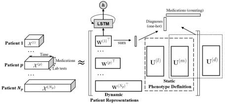
In this section, we describe the framework of our pro-posed model to jointly learn the static phenotype defini-tions and the patient-specific dynamic representation. We start from the collective non-negative tensor factorization (CNTF), which models each patient with a temporal ten-sor to avoid aligning patients with different temporal length. Then we demonstrate the flexibility of the proposed ba-sic model where non-temporal data modalities without time stamps can also be readily incorporated. Finally, we intro-duce an RNN-based regularization to better model the tem-poral relationship. The overview of the proposed framework is illustrated in Fig. 1.
Collective Non-Negative Tensor Factorization
Given a collection of patient records withKmodalites that are recorded with time stamps, we aim to simultaneously discover the static phenotype definitions describing the true disease states and the dynamic representation of the patients revealing the dynamic changes of the disease states of the patients throughout the observation window. The length of the observation window for each individual patient may dif-fer from each other. For instance, if the observation window is a hospital stay, it is not feasible to construct a single tensor for all patients as most of the existing models do due to the inconsistency of the time dimension. Instead, we construct a (K+ 1)thorder interaction tensor for each patient, resulting a collection ofNptemporal tensors,i.e.X={X(p)|X(p)∈ RTp×I1×···×IK, forp= 1, . . . , Np}, whereNp is the num-ber of patients,X(p) is the temporal tensor for thepth pa-tient,Tp is the temporal length of thepthpatient’s records andIkis the size of thekthdimension. Without loss of gen-erality, we assumeK = 2 with the dimensions being lab testsandmedicationsrespectively for simplifying the nota-tions. As presented in the previous section, the non-negative
Figure 1: The framework of the proposed model. A3rdorder time-labtest-medication tensor is constructed for each pa-tient, and all of the temporal tensors are factorized with the phenotype definitions being shared across all the patients. RNN-based regularization is introduced to model the time dependency of the dynamic patient representations. Another tensor model called HITF (Yin et al. 2018) is also incorpo-rated to allow non-temporal modalities to be utilized.
CP factorization of the3rdorder temporal tensor yields three latent factor matricesW(p) ∈
RTp×R,U(l) ∈
RIl×Rand
U(m) ∈
RIm×R, whereRis the number of phenotypes,Il is the number of lab tests and Im is the number of med-ications. We refer to the latter two factor matrices as the phenotype definitions. In order to discover phenotypes that account for all patients rather than a single patient, we intro-duce the hard constraint thatU(k)has to be shared across all
patients for allk. The first factor matrixW(p)is referred to
as dynamic patient representation because its entryw(trp) de-scribes how likely therthphenotype exists at the particular time pointt. We may understand this, intuitively, as learn-ing a “dictionary” that describes some potentially clinically meaningful disease states, and concurrently selecting differ-ent non-negative combinations of these disease states for dif-ferent patients at difdif-ferent time points to approximate the in-put data. The formulation of the CNTF model with lab tests and medications is given in Eq. 3.
arg min W(p),U(l),U(m)
fCNTF≡
Np
X
p=1
1
Tp
X
ijk b
xijk(p)−xijk(p)logxb(ijkp)
subject to Xb
(p)
=JW(p),U(l),U(m)K ∀p
W(p)≥0 ∀p,
(3)
U(l)≥0,U(m)≥0,
where the loss function is given by the weighted sum of that of factorizing each individual temporal tensor. To pre-vent the total loss being dominated by samples with very long temporal lengths, the individual loss of each sample is weighted by the reciprocal of its temporal length.
The advantages of the proposed schema are twofold.
• Revealing patient-specific dynamic patterns.Even if a 4thorder tensor can be constructed, factorizing the tensor with time dimension yields temporal factors that account for the global evolution across all data samples (Xiong et al. 2010). Although this could be advantageous under some particular scenarios, we believe it would be prefer-able to make the temporal factorspecificfor each patient since the disease progression could be very distinct for different individuals, even with the same diagnoses.
To illustrate the second point in more detail, let us assume that a4thorder tensorX0 with size ofN
p×Tp×Il×Im can be constructed with its CP factors for the four dimen-sions being W0, U(t), U(l) and U(m) respectively. Then we havex0pijk =PR
r=1w
0
pru (t) iru
(l) jru
(m)
kr , wherew
0
pru (t) ir is the patient loading and can be interpreted as the probability of phenotype rbeing existent for patient pat time iafter proper re-scaling. It clearly follows that the patient loading vector over time is essentially thegloballyshared temporal factors weighted by a patient-specific scalarw0pr, resulting the disease progression for all patients following the same dynamic pattern with different amplitude. To the contrary, it is straightforward that the proposed CNTF model reveals the dynamic patterns specific for each individual patient.
Incorporating Non-temporal Data Modality
It is often the case that some data types do not have time stamps. For example, in MIMIC-III dataset (Johnson et al. 2016), the diagnosis codes are generated upon patient dis-charge for the billing purpose. Thus the time of making diag-nosis is not available. Yet the diagdiag-nosis information is very useful for discovering clinically meaningful phenotypes. We integrate the diagnosis by adopting the Hidden Interaction Tensor Factorization (HITF) model proposed in (Yin et al. 2018). The HITF model is derived based on the accumula-tion of diagnoses and medicaaccumula-tions over the observaaccumula-tion win-dow. It takes apatient-by-medicationcounting matrix and a patient-by-diagnosisbinary matrix as input, and computes the CP factorization of the hidden tensor describing the in-teractions among the medications and diagnoses. For thepth patient, we sum up the patient representationW(p)along the time dimension as the representation for the whole observa-tion window. The input then would be a medicaobserva-tion vectorm
indicating what and how many medications are prescribed to thepthpatient and a binary diagnosis vectordindicating the diagnoses assigned to the patient. We rewrite the formulation of the HITF model for an individual patient as follows:
arg min W(p),U(d),U(m)
fpHITF ≡X
i ˆ
d(ip)−di(p)log(edˆ(ip)−1)+
X
j ˆ
mj(p)−mj(p)log ˆm(jp)
subject to dˆ(p)=e>W(p)diag(e>U(m))U(d)>
(4)
ˆ
m(p)=e>W(p)diag(e>U(d))U(m)> W(p)≥0,U(m)≥0,U(d)≥0.
RNN-based Temporal Regularization
Although the temporal relationship can be captured byW(p)
as described earlier, the temporal dependency of the dis-ease state over time is not explicitly modeled, implying each time point being treated independently. However, the inde-pendence assumption is not appropriate here for the time dimension, as it does not take into account the ordering of the clinical events, which is inherently important for medi-cal applications. In order to model the temporal dependency, we propose to make use of an RNN which is recently pre-dominant for time series and sequential data analysis. With the dynamic patient representations being learned, we may regard eachW(p)as a multi-variable time series with each
variable describing the progression of the existence of the corresponding phenotype for patientp. Given the time series prior to timet,i.e.w1, . . . ,wt−1where we omit the
super-script(p)and subscriptrdenoting the patient and phenotype respectively, we use the RNN model to predictwtand min-imize the Mean Square Error (MSE) between the real and predicted value. The regularization term is written as:
R(W(p)) = 1 Tp
Tp
X
t=2
g(wt−1)−wt
2
2, (5)
whereg(wt−1)is the prediction output given by the RNN
model. In this work, we use a two-layer LSTM net-work (Hochreiter and Schmidhuber 1997) with200hidden units as the RNN model.
As a regularization, the RNN model is jointly learned with the CNTF model. Intuitively, the RNN model captures the temporal dependency with its hidden units, and then the pa-tient representationW(p)is updated so that the recovery
er-ror of the CNTF model and the temporal predictive MSE loss together is minimized, enforcing the patient represen-tation being mostly consistent with the regularity captured by the LSTM network as well as recovering the temporal tensor.
Learning Algorithms
The final loss function is given by the weighted sum of the CNTF loss, the HITF loss and the temporal regularization loss as follows:
`=α1fCNTF+α2 Np
X
p=1
fHITF
p +β
Np
X
p=1
R(W(p)), (6)
where the variablesW(p) ∀p,U(l)andU(m)have to satisfy the non-negativity constraints. To ease the parameter tuning, α1is fixed to one throughout all the experiments.
The medication vector used in HITF model is the accu-mulation of the entire hospital visit. Thus, intuitively, em-phasizing the HITF loss too much (largeα2) would possibly
hinder the medications used at different disease stages be-ing well separated, while a too smallα2could fail to capture
We adopt the block coordinate descent optimization framework and mini-batch projected gradient descent to solve the problem. In each mini-batch, we first sample m data points{X(i)|i∈ L}with theLbeing the data point
in-dices. Then, we updateU(l)andU(m)in turn with all other
variables fixed, followed by updatingW(i) ∀i∈ L. Lastly,
we feedW(i)∀ias input to the LSTM network and update it
using the standard back-propagation. The optimization pro-cedure is summarized in Algorithm 1.
Algorithm 1: Optimization Framework for Solving LSTM Regularized CNTF Model
Input :time-labtest-medicationtensor collection:
{X(p)|X(p)∈
RTp×Il×Im, p= 1, . . . , N
p}, medication vectors:{m(p), p= 1, . . . , Np}, diagnosis vectors:{d(p), p= 1, . . . , Np}, model parameters:α1, α2andβ. Output:patient representations:W(p) ∀p,
phenotype definitions:U(l),U(m)andU(d).
1 initialization; 2 foreach epochdo 3 foreach mini-batchdo
4 sample mini-batch ofmtensors and vectors from input with indicesL;
5 forX∈ {U(l),U(m),U(d)}do
6 updateXby descending its stochastic gradient; 7 non-negative projection byX←max(0,X); 8 end
9 fori∈ Ldo
10 updateW(i)by descending its stochastic
gradient;
11 non-negative projection by
W(i)←max(0,W(i)); 12 end
13 update LSTM model by back-propagation; 14 end
15 end
The time complexity of the CNTF model remains the same with formulating as a 4th order tensor factorization problem, but in practice the CNTF model is more efficient because solving forW(i)is independent of each other with
all other variables fixed, and the gradientw.r.t.U(l),U(m)
andU(d) can be computed by summing up the gradient of
each individual data sample, thus allowing them to be easily parallelized.
Experiments and Results
We conduct the experiments on a real-world Intensive Care Units (ICU) dataset, MIMIC-III, where the quality of the inferred phenotypes is evaluated. Furthermore, we use the inferred phenotypes as features for the mortality prediction task and evaluate the classification accuracy.
Data Set
Medical Information Mart for Intensive Care (MIMIC-III) (Johnson et al. 2016) is a large-scale, open-source and
de-identified ICU dataset, containing records related to over forty thousand patients who stayed in the ICU at Beth Israel Deaconess Medical Center between 2001 and 2012. In this paper, we focus on the medication prescriptions, of which the prescription date and duration dates are recorded, and the laboratory test results with time stamps recorded. Since many laboratory tests are requested and performed repeat-edly in ICU, we only use the abnormal laboratory test events to avoid the frequent normal laboratory results dominat-ing the input tensor. We construct a3rdorder time-labtest-medication binary interaction tensor X(p) for patient pby
setting the tensor entryx(tijp)to be one if the abnormal labtest eventiand the medication eventjco-occur at time t. The time resolution is one day. We extract a subset of MIMIC-III dataset containing4,590adult patients with length-of-stay longer than7days, and50%of them deceased in the hospi-tal. We also exclude the base type drugs,e.g.D5W, and use the top300most frequent medications. The diagnosis codes are generated upon patient discharge by reviewing the clini-cal notes during the hospital stay, and thus the exact time of the diagnoses being assigned is not available. We group the diagnoses by the first three digits of their ICD-9 codes and use the top300most frequent diagnoses.
Phenotypes
The primary task of computational phenotyping is to derive clinically meaningful and interpretable phenotypes that cor-respond to some true disease states. Thus, we first evaluate the quality of the learned phenotypes. In order to include diagnoses in the phenotypes to enhance the interpretability, the HITF model is incorporated as described in Eq. 4, and the weightingα2is set to0.05. The number of phenotypes
is set to 50. The RNN regularization is switched on with weightβset to10.
Table 1 shows three phenotypes derived by our proposed model. It can be seen that the inferred phenotypes corre-spond to different disease states in ICU, which is endorsed by a medical expert. Phenotype 1 corresponds to the di-agnosis, Chronic Kidney Disease (CKD) and the identified abnormal laboratory tests, especially the RBC (Red Blood Cells) in urine, blood osmolality and protein/creatinine ra-tio in urine. In the clinical context, the disease state CKD is indeed associated with elevated RBC in urine due to renal tubular necrosis, elevated blood osmolality due to electrolyte retention in the vascular system, and elevated protein loss in the urine leading to an abnormal protein/creatinine ratio. Phenotype9corresponds to the diagnosis Other Disease of the Lung and abnormal laboratory tests pO2, pCO2, pH of the arterial blood gas. Again, this correlates well with the clinical context, where reduced oxygen levels and pH, and elevated carbon dioxide levels all indicate the presence of acute respiratory failure (which is classified under the “other disease of lung” in the ICD-9 coding system).
Phenotype 1 Phenotype 4 Phenotype 9
Chronic kidney disease (CKD) (0.536)
Other forms of chronic ischemic heart disease (0.507) Cardiac dysrhythmias (0.372) Essential hypertension (0.024)
Other diseases of lung (0.876)
RBC (Urine) (0.200)
Osmolality, Measured (Blood) (0.117) Protein/Creatinine Ratio (Urine) (0.069)
Hematocrit (Blood) (0.072) Red Blood Cells (Blood) (0.071)
Hemoglobin (Blood) (0.070)
pO2 (Blood Gas) (0.253) pCO2 (Blood Gas) (0.237)
pH (Blood Gas) (0.215) Hydromorphone (0.336)
Phenylephrine (0.038) Aspirin (0.033)
Acetaminophen (0.188) Metoclopramide (0.102) Insulin Human Regular (0.070)
Acetaminophen (0.113) Insulin (0.099) Bisacodyl (0.089)
Table 1: Three examples of the learned phenotypes. The rows correspond to diagnoses, abnormal laboratory results and med-ications respectively, where the numbers between parentheses are the weightings. Due to space limitation, only the first three items are listed.
Phenotype 1 Phenotype 2 Phenotype 3
Other diseases of lung (0.045) Septicemia (0.040) Certain adverse effects not elsewhere classified (0.039)
Other diseases of lung (0.040) Acute kidney failure (0.036)
Certain adverse effects not elsewhere classified (0.032)
Acute kidney failure (0.039) Other diseases of lung (0.037)
Cardiac dysrhythmias (0.033)
Glucose(Blood) (0.019) Red Blood Cells(Blood) (0.019)
Hematocrit(Blood) (0.019)
Hematocrit(Blood) (0.017) Red Blood Cells(Blood) (0.017)
Glucose(Blood) (0.017)
Glucose(Blood) (0.018) Hematocrit(Blood) (0.018) Red Blood Cells(Blood) (0.018) Vancomycin (0.017)
Insulin (0.015) Potassium Chloride (0.015)
Vancomycin (0.013) Potassium Chloride (0.013) Pantoprazole Sodium (0.012)
Vancomycin (0.015) Potassium Chloride (0.014)
Heparin (0.014)
Table 2: Three examples of the phenotypes derived by the Rubik model. The rows correspond to diagnoses, abnormal laboratory results and medications respectively. Due to space limitation, only the first three items are listed.
Table 2 shows the phenotypes derived by the Rubik model, where we can see that the weightings of the clinical items within each phenotype are widely distributed, instead of concentrating on some specific items. The inferred pheno-types all correspond to some complex, critical and possi-bly end-stage disease states, including the diagnoses of sep-ticemia and acute kidney failure, and medication of van-comycin which is often used in ICU for treatment of life-threatening infections by Gram-positive bacteria that are unresponsive to other antibiotics. Moreover, the identified abnormal laboratory tests are very general, which do not specifically relate to either the diagnoses or the medications.
The comparison between the phenotypes derived by our proposed CNTF model and the Rubik model reveals that it is extremely difficult to separate the disease states appearing at different stages of the patient journey given the input ten-sor being accumulated over the observation window. With our proposed CNTF model; however, the different disease states occurring at different time points could be discovered, reflected by the fact that the chronic diseases, such as CKD, can be captured with meaningful combinations of medica-tions and abnormal laboratory tests. Therefore, we conclude that our proposed CNTF model infers significantly more in-terpretable and clinically meaningful phenotypes than the baseline.
Sparsity Similarity
Rubik 0.79 0.90
CNTF 0.96 0.43
Table 3: Sparsity and similarity of phenotypes derived by the proposed CNTF model and the baseline Rubik model.
Sparsity and Similarity
Sparsity and similarity are two commonly used proxy met-rics for measuring the interpretability of the derived pheno-types quantitatively (Kim et al. 2017; Yin et al. 2018). The sparsity is defined by the ratio of zero elements in the phe-notype definition matrices, and the similarity is defined as the average cosine similarity score given by:
Similarity Score=
P
k
PR
r1
PR
r2>r1 n
cos(U(:rk1),U (k) :r2)
o
Figure 2: Visualization of three examples of the dynamic pa-tient representations. Each row corresponds to a phenotype, and the grey level indicates the weighting of the phenotype at different time points (normalized by the maximum value of each row). The definitions of phenotype 1, 4 and 9 are given in Table 1, and that of the remaining phenotypes are given in the supplemental material.
Interpretation of the Dynamic Patient
Representations
As described earlier, the dynamic patient representation
W(p)indicates the evolution of the disease states over the observation window. With meaningful phenotypes being in-ferred, we anticipate that the patient representations are also highly interpretable. Fig. 2 shows the visualization of three examples of the dynamic patient representations learned to-gether with the phenotype definitions. Each sub-figure corre-sponds to one individual patient, where each row within each sub-figure corresponds to one particular phenotype, and the grey level of each cell indicates the strength of the corre-sponding phenotype being present at that time. We normal-ize the values by the maximum value of each row for better visual effect.
We presented the visualization to a medical expert for qualitative evaluation. According to the expert, the learned patient representations are highly interpretable. The first ex-ample patient has phenotype 4, which corresponds to the dis-ease “Chronic Heart Disdis-ease”, with high values in the first several days and decreasing in the remaining of the hospi-tal stay. This suggests that the lab tests and medications are related to this disease entity only during the initial few days of the ICU stay. This patient’s data then goes on to demon-strate high values for phenotypes 3, 5, 7 and 11, which corre-spond to Other Disease of the Lung, Cardiac Dysrhythmias, Acute Kidney Failure, and Cardiac Dysrhymias with Heart Failure, respectively. Essentially, the data describe a clinical scenario in which the patient is admitted with a problem re-lated to an existing condition (chronic heart disease) which is treated unsuccessfully, so the patient deteriorates and
de-Figure 3: Prediction accuracy of in-hospital mortality at dif-ferent time
velops multiple organ failure (lung, heart, kidney failure). Indeed, closer review of the clinical textual documentation of this patient shows that the aforementioned scenario does closely correlate with what actually occurred.
Mortality Prediction Task
We further evaluate the derived phenotypes by performing an in-hospital mortality prediction task using the derived phenotypes as features. We split the data into training set and test set with a proportion of8 : 2. The phenotypes are de-rived based on the training set, which is totally unsupervised. Then we fix the learned phenotype definitions and project the test set onto the learned phenotypes to obtain the patient representation for the test set. Finally we use a lasso regular-ized logistic regression to perform the binary classification. We measure the AUROC on different days in an accumu-lated manner,e.g., the AUROC value for the second day is obtained by considering the patient representations within the first two days. The HITF model is switched off by set-ting α2 in Eq. 6 to zero for this task since the diagnoses
codes are only available after discharge. We avoid using di-agnosis codes for making predictions prior to discharge to ensure fair evaluation.
baselines cannot. This also validates that CNTF can infer phenotypes that correspond to more specific disease states, rather than mixtures of different disease states. Finally at discharge, all models achieve AUROC of 0.85, which is not surprising since the patients can be well represented by the baseline phenotype given the data accumulated over the whole hospital stay.
Conclusion
In this paper, we present a novel Collective Non-negative Tensor Factorization (CNTF) model to simultaneously learn the dynamic patient representations that are specific for each individual patient, and the phenotype definitions that are shared across all the patients. The proposed model takes into account the varying length of the patient records by form-ing a temporal tensor for each patient, the non-temporal data modalities by incorporating the HITF model, and the tempo-ral dependency of the disease states by introducing an RNN-based regularization.
The experimental results demonstrate that the pheno-types inferred by CNTF are clinically meaningful and inter-pretable, and correspond to different specific disease states that occur at different times of the patient journey, which cannot be easily obtained by the baseline model with the in-put tensor being accumulation over the observation window. Moreover, this is also validated by the significant predictive performance boost in the early stage of the hospital admis-sion. For future research directions, we will focus on utiliz-ing data with different temporal resolutions to discover more clinically relevant phenotypes.
Acknowledgments
This research is partially supported by General Research Fund 12202117 from the Research Grants Council of Hong Kong.
References
Che, Z.; Purushotham, S.; Cho, K.; Sontag, D.; and Liu, Y. 2018. Recurrent neural networks for multivariate time series with missing values.Scientific Reports8(1):6085.
Chi, E. C., and Kolda, T. G. 2012. On tensors, sparsity, and non-negative factorizations.SIAM Journal on Matrix Analysis and Ap-plications33(4):1272–1299.
Choi, E.; Bahadori, M. T.; Schuetz, A.; Stewart, W. F.; and Sun, J. 2016a. Doctor AI: Predicting clinical events via recurrent neural networks. InMachine Learning for Healthcare Conference, 301– 318.
Choi, E.; Bahadori, M. T.; Sun, J.; Kulas, J.; Schuetz, A.; and Stew-art, W. 2016b. RETAIN: An interpretable predictive model for healthcare using reverse time attention mechanism. InAdvances in Neural Information Processing Systems, 3504–3512.
Henderson, J.; Ho, J. C.; Kho, A. N.; Denny, J. C.; Malin, B. A.; Sun, J.; and Ghosh, J. 2017. Granite: Diversified, sparse tensor fac-torization for electronic health record-based phenotyping. In2017 IEEE International Conference on Healthcare Informatics (ICHI), 214–223. IEEE.
Ho, J. C.; Ghosh, J.; Steinhubl, S. R.; Stewart, W. F.; Denny, J. C.; Malin, B. A.; and Sun, J. 2014. Limestone: High-throughput
can-didate phenotype generation via tensor factorization. Journal of Biomedical Informatics52:199–211.
Ho, J. C.; Ghosh, J.; and Sun, J. 2014. Marble: high-throughput phenotyping from electronic health records via sparse nonnegative tensor factorization. InProceedings of the 20th ACM SIGKDD In-ternational Conference on Knowledge Discovery and Data Mining, 115–124. ACM.
Hochreiter, S., and Schmidhuber, J. 1997. Long short-term mem-ory. Neural Computation9(8):1735–1780.
Hripcsak, G., and Albers, D. J. 2013. Next-generation phenotyp-ing of electronic health records. Journal of the American Medical Informatics Association20(1):117–121.
Johnson, A. E.; Pollard, T. J.; Shen, L.; Li-wei, H. L.; Feng, M.; Ghassemi, M.; Moody, B.; Szolovits, P.; Celi, L. A.; and Mark, R. G. 2016. MIMIC-III, a freely accessible critical care database.
Scientific Data3:160035.
Kim, Y.; El-Kareh, R.; Sun, J.; Yu, H.; and Jiang, X. 2017. Dis-criminative and distinct phenotyping by constrained tensor factor-ization.Scientific Reports7(1):1114.
Kirby, J. C.; Speltz, P.; Rasmussen, L. V.; Basford, M.; Gottesman, O.; Peissig, P. L.; Pacheco, J. A.; Tromp, G.; Pathak, J.; Carrell, D. S.; et al. 2016. PheKB: a catalog and workflow for creating electronic phenotype algorithms for transportability.Journal of the American Medical Informatics Association23(6):1046–1052. Kolda, T. G., and Bader, B. W. 2009. Tensor decompositions and applications.SIAM Review51(3):455–500.
Lee, D. D., and Seung, H. S. 1999. Learning the parts of objects by non-negative matrix factorization.Nature401(6755):788. Perros, I.; Papalexakis, E. E.; Wang, F.; Vuduc, R.; Searles, E.; Thompson, M.; and Sun, J. 2017. SPARTan: Scalable PARAFAC2 for large & sparse data. InProceedings of the 23rd ACM SIGKDD International Conference on Knowledge Discovery and Data Min-ing, 375–384. ACM.
Purushotham, S.; Meng, C.; Che, Z.; and Liu, Y. 2018. Benchmark-ing deep learnBenchmark-ing models on large healthcare datasets. Journal of Biomedical Informatics.
Wang, Y.; Chen, R.; Ghosh, J.; Denny, J. C.; Kho, A.; Chen, Y.; Malin, B. A.; and Sun, J. 2015. Rubik: Knowledge guided ten-sor factorization and completion for health data analytics. In Pro-ceedings of the 21th ACM SIGKDD International Conference on Knowledge Discovery and Data Mining, 1265–1274. ACM. Xiong, L.; Chen, X.; Huang, T.-K.; Schneider, J.; and Carbonell, J. G. 2010. Temporal collaborative filtering with Bayesian prob-abilistic tensor factorization. InProceedings of the 2010 SIAM International Conference on Data Mining, 211–222. SIAM. Yadav, P.; Steinbach, M.; Kumar, V.; and Simon, G. 2018. Min-ing electronic health records (EHRs): a survey. ACM Computing Surveys (CSUR)50(6):85.
Yang, K.; Li, X.; Liu, H.; Mei, J.; Xie, G.; Zhao, J.; Xie, B.; and Wang, F. 2017. TaGiTeD: Predictive task guided tensor decom-position for representation learning from electronic health records. InProceedings of the Thirty-First AAAI Conference on Artificial Intelligence.
Yin, K.; Cheung, W. K.; Liu, Y.; Fung, B. C. M.; and Poon, J. 2018. Joint learning of phenotypes and diagnosis-medication correspon-dence via hidden interaction tensor factorization. InProceedings of the Twenty-Seventh International Joint Conference on Artificial Intelligence, 3627–3633.
Yu, H.-F.; Rao, N.; and Dhillon, I. S. 2016. Temporal regularized matrix factorization for high-dimensional time series prediction. In