Improving Optimization Bounds Using Machine Learning: Decision Diagrams Meet Deep Reinforcement Learning

(1)

The Thirty-Third AAAI Conference on Artificial Intelligence (AAAI-19)

Improving Optimization Bounds Using Machine

Learning: Decision Diagrams Meet Deep Reinforcement Learning

Quentin Cappart,

1

Emmanuel Goutierre,

2

David Bergman,

3

Louis-Martin Rousseau

1 1_{Ecole Polytechnique de Montr´eal, Montr´eal, Canada}

2_{Ecole Polytechnique, Paris, France}

3_{University of Connecticut, Stamford, CT 06901, USA}

{quentin.cappart, louis-martin.rousseau}@polymtl.ca [email protected]

[email protected]

Abstract

Finding tight bounds on the optimal solution is a critical el-ement of practical solution methods for discrete optimiza-tion problems. In the last decade, decision diagrams (DDs) have brought a new perspective on obtaining upper and lower bounds that can be significantly better than classical bound-ing mechanisms, such as linear relaxations. It is well known that the quality of the bounds achieved through this flexible bounding method is highly reliant on the ordering of variables chosen for building the diagram, and finding an ordering that optimizes standard metrics is an NP-hard problem. In this pa-per, we propose an innovative and generic approach based on deep reinforcement learning for obtaining an ordering for tightening the bounds obtained with relaxed and restricted DDs. We apply the approach to both the Maximum Inde-pendent Set Problem and the Maximum Cut Problem. Ex-perimental results on synthetic instances show that the deep reinforcement learning approach, by achieving tighter objec-tive function bounds, generally outperforms ordering meth-ods commonly used in the literature when the distribution of instances is known. To the best knowledge of the authors, this is the first paper to apply machine learning to directly im-prove relaxation bounds obtained by general-purpose bound-ing mechanisms for combinatorial optimization problems.

Introduction

Relaxation bounds, and mechanisms by which those bounds can be improved, are perhaps the most critical element of scalable generic algorithms for discrete optimization prob-lems. As machine learning popularizes, a natural question arises: how can machine learning be used for improving op-timization bounds ? Finding a way to utilize the power of machine learning to prove tighter relaxation bounds may be a key for unlocking significant performance improve-ments in optimization solvers. This paper provides, to the best knowledge of the authors, a first effective approach in the literature towards achieving this goal.

The challenge one faces in using machine learning to tighten relaxation bounds is that the bound provided by clas-sical methods (e.g., LP or SDP relaxations) areinflexible; the algorithm used to solve the relaxation has no effect on

the quality of the bound. For example, given an IP model, the LP relaxation will report the same bound independent of what method is used to solve the relaxation and any other decision employed during the solution algorithm.

Contrastingly, approximate decision diagrams (DDs) (Bergman, van Hoeve, and Hooker 2011), a recently intro-duced optimization technology, provide aflexiblebounding method, in that decisions employed in the execution of the algorithms used to build the DDs directly affect the quality of the bound. This is true for both relaxed DDs, that prove relaxation bounds, and restricted DDs, that identify primal solutions. This opens the door for potential integration with machine learning.

Initially introduced for representing switching circuits (Lee 1959) and for formal verification (Bryant 1986), DDs in discrete optimization are used to encode the feasible solu-tions of a problem while preserving its combinatorial struc-ture. A common application is to provide bounds, both up-per and lower, for discrete optimization problems (Bergman, van Hoeve, and Hooker 2011; Bergman et al. 2013). How-ever, the quality of the bounds is known to be tightly related to the variable ordering considered during the construction of the DD (Bergman et al. 2012). It has been shown that find-ing an optimal orderfind-ing for general DDs is NP-hard and is often challenging to even model. Besides, improving a given variable ordering is known to be NP-complete (Bollig and Wegener 1996). Thus, designing methods for finding a good ordering is a hot topic in the community and continues as a challenge. The idea suggested in this paper is to use machine learning to identify good variable orderings that therefore re-sult in tighter objective function bounds.

(2)

The main issue is that some states are never considered dur-ing the learndur-ing process when large state spaces are consid-ered. Recently, deep learning (LeCun, Bengio, and Hinton 2015) provided new tools to overcome this problem. The idea is to use a deep architecture as a function approxima-tion for generalizing knowledge from visited to unknown states. Such an improvement enabled RL to scale to prob-lems that were previously intractable. Notorious examples are the superhuman performances obtained for the game of Go (Silver et al. 2016) and Atari 2600 (Mnih et al. 2013; Mnih et al. 2015). The combination of RL with a deep net-work is commonly referred asdeep reinforcement learning (DRL) (Arulkumaran et al. 2017).

Even more recently, DRL has also been applied to iden-tify high-quality primal bounds to some NP-hard combina-torial problems. Most work focuses on the classical Trav-eling Salesman Problem (Bello et al. 2016; Deudon et al. 2018), with the exception of the approach of Khalil et al. (Khalil et al. 2017) that tackles four NP-hard problems hav-ing a graph structure. They use a deep learnhav-ing architecture in order to embed the graph structure into features (Dai, Dai, and Song 2016). The competitive results obtained suggest that this approach is a promising new tool for finding so-lutions to NP-hard problems. In this paper, we further push these efforts to be able to generate dual bounds.

Given this related work, our contribution is positioned as follows. We propose a generic approach based on DRL in order to identify variable orderings for approximate DDs. The goal is to find orderings providing tight bounds. The fo-cus is on relaxed DDs, as this provides a mechanism for uti-lizing machine learning to improve relaxation bounds, but we also show the effectiveness for restricted DDs, adding to the recent literature on using machine learning for find-ing high-quality heuristic solutions. The approach has been validated on the Maximum Independent Set Problem, for which the variable ordering has been intensively studied (Bergman et al. 2012). Its application to the Maximum Cut Problem is also considered. We note that there has been lim-ited work on applying machine learning to identify vari-able orderings for DDs in unrelated fields (Carbin 2006; Grumberg, Livne, and Markovitch 2011). To the best of our knowledge, this work has not been extended to optimization. This paper is structured as follows. The next section intro-duces the technical background related to DDs and RL. The process that we designed for learning an appropriate variable ordering is then presented. The RL model and the learning algorithms are detailed and the construction of the DD using RL is described. Finally, experiments on synthetic instances are carried out in the last section.

Technical Background

Decision Diagrams

In the optimization field, adecision diagram(DD) is a struc-ture that encodes a set of solutions to a constrained opti-mization problem (COP)⟨X, D, C, O⟩whereXis the set of variables,Dthe set of discrete domains restricting the val-ues that variablesx∈Xcan take,Cthe sets of constraints andOthe objective function. Formally, a DD associated to a

combinatorial problemPis a directed-layered-acyclic graph

BP = ⟨U, A, d⟩whereU is the set of nodes,A the set of arcs anddis a functionA →Nassociating a label at each

arc. The set of nodes U is partitioned into layersLi, i.e.,

U = ∪m

i=1Li. LayersL1 andLm are both composed of a single node: the root and the terminal node, respectively. The widthwi(B)of layerLiin a DDBis defined as the number of nodes in that layer:wi(B) = |Li|. The width w(B)of the DD is the maximum-width layer:w(B) = maxiwi(B). Each arca ∈ Ais directed from a node in a layerLi to a node in layer Li+1 wherei ∈ [0, m−1]. The function d

associates to each arcaalabeld(a). The arcs directed out of each nodeu∈U have distinct labels, i.e., at most one arc with tailahaving any domain valued. We assume that for eachu, there must exist a directed path from the root node touand fromuto the terminal node. Acostc(a) ∈ _Ris also associated to every arc ina, which is used to encode the objective function of solutions.

In this paper, a DDBPfor a COPPhasn+1layers where nis the number of decision variables inP. Each layerLi (except the last one) is linked to one variablexiofP and an arcafromLitoLi+1with labeld(a)represents the

assign-mentxitod(a). A direct path from the root to the terminal node ofBPcorresponds then to a solution ofP. The assign-ment of variables inP to layers during the construction of the DD is referred as thevariable ordering.

A DD is exact when the solutions encoded align ex-actly with the feasible solutions of the initial problem P

and for any arc-directed root-to-terminal node path p, the sum of the costs of the arcs equates to the evaluation of the objective function for the solutionxit corresponds, i.e.,

∑

a∈pc(a) = O(x). In this case, the longest path (assum-ing a maximization problem) from the root to the terminal node corresponds to the optimal solution ofP. However, the width of DDs tends to grow exponentially with the number of variables in the problem, which reduces its usability for large instances. A DD isrelaxedwhen its encodes a superset of the feasible solutions ofP and for any arc-directed root-to-terminal node pathp, the sum of the costs of the arcs is an upper bound (still in the case of a maximization problem) on the evaluation of the objective function for the solutionxit corresponds, i.e.,∑

a∈pc(a)≥O(x). A relaxed DD can be constructed incrementally, merging nodes on each layer un-til the width is below a threshold (Bergman, van Hoeve, and Hooker 2011) in such a way that no solution is lost during the merging process. Hence, for a relaxed DD, the longest path gives an upper bound of the optimal solution forP. Fi-nally, a DD isrestrictedwhen it under-approximates the fea-sible solutions ofPand for any arc-directed root-to-terminal node pathp, the sum of the costs of the arcs is a lower bound on the evaluation of the objective function for the solutionx

it corresponds, i.e., ∑

(3)

and restricted DDs. Both take as input a specified maximum width, and it has been empirically shown that larger DDs generally provide tighter bounds but are in return more ex-pensive to compute. An exhaustive description of DDs and their construction are provided in (Bergman et al. 2016).

Reinforcement Learning

Let⟨S, A, T, R⟩be a tuple representing a deterministic cou-ple agent-environment where S is the set of states in the environment, A the set of actions that the agent can do,

T : S ×A → S the transition function leading the agent from a state to another one given the action taken and

R : S×A → R the reward function of taking an action

from a specific state. The behavior of an agent is defined by a policyπ:S→A, describing the action to be done given a specific state. The goal of an agent is to learn a policy max-imizing the accumulated sum of rewards (eventually dis-counted) during its lifetime defined by a sequence of states

st∈Switht∈[1,Θ]. Such a sequence is called anepisode wheresΘis the terminal state. The expected return after time

steptis denoted byGt=∑Θ_k₌_t₊₁γk−t−1R(sk, ak)where γ∈[0,1]is a discounting factor used for parametrizing the weight of future rewards. For a deterministic environment, The quality of taking an actionafrom a statesunder a pol-icyπis defined by the action-value functionQπ(s, a) =Gt. The problem is to find a policy maximizing the expected re-turn:π⋆ = argmaxπQπ(s, a)∀s∈S,∀a∈A. In practice, π⋆_{is computed from an initial policy and by two nested} op-erations: (1) the policy evaluation, making the action-value function consistent with the current policy, and (2) the policy iteration, improving greedily the current policy.

However, in practice, the optimal policy, or even an op-timal action-value function, cannot be computed in a rea-sonable amount of time. A method based on approximation, such as Q-learning (Watkins and Dayan 1992), is then re-quired. Instead of computing the optimal action-value func-tion, Q-learning approximates the function by iteratively updating a current estimate after each action. The update function is defined as follows: Q(st, at)

α

←− R(st, at) + γmaxa∈AQ(st+1, a), where x

α

←− y denotes the update

x←x+α(y−x)andα∈(0,1]the learning rate. Another issue arising for large problems is that almost every state encountered may never have been seen during previous updates, thus necessitating a method capable of utilizing prior knowledge to generalize for different states that share similarities. Among them, neural fitted Q-learning (Riedmiller 2005) uses a neural network for approximat-ing the action-value function. This provides an estimator

ˆ

Q(s, a,w) ≈ Q(s, a) wherew is a weight vector that is learned. Stochastic Gradient Descent (Bottou 2010) or an-other optimizer coupled with back-propagation (Rumelhart, Hinton, and Williams 1986) is then used for updating w and aims to minimize the squared loss between the cur-rent Q-value and the new value that should be assigned us-ing Q-learnus-ing: w ← w − 1

2α∇L(w) where the square

loss is L(w) = (

R(st, at) +γmaxa∈AQˆ(st+1, a,w)−

ˆ

Q(s, a,w))2. Updates are done usingexperience replay. Let

⟨s, a, r⟩be a sample representing an action done at a spe-cific state with its reward andDa sample store. Each time an action is performed,⟨s, a, r⟩is added inD. Then, the op-timizer updateswusing a random sample taken fromD.

Learning Process

Reinforcement Learning Formulation

Designing a RL model for determining the variable order-ing of a DD associated to the COP ⟨X, D, C, O⟩requires defining, adequately, the tuple⟨S, A, T, R⟩to represent the system. Our model is defined as follows.

State A states∈Sis a pair⟨sL, sB⟩containing an ordered sequence of variablessL and a partially constructed DD sBassociated with variables insL. A statesis terminal if sLincludes all the variables ofX.

Action An action is defined as the selection of a variable fromX. An actionascan be performed at statesif and only if it is not yet inserted insB(as∈X\sL).

Transition A transition is a function updating a state ac-cording to the action performed. LetB⊕xbe an operator adding the variablexinto a decision diagramBandy::x

another operator appending the variablexto the sequence

y, we haveT(s, as) =⟨sL::as, sB⊕as⟩.

Reward The reward function is designed to tighten the bounds obtained with the DD. When maximizing, upper bounds are provided by relaxed DDs and lower bounds by restricted DDs. Both cases are associated with a com-mon reward. Let ⌈B⌉ and⌊B⌋indicate the current up-per/lower bound obtained with the DD B. Such bounds correspond to the current partial longest path of the re-laxed/restricted DD from the root node to the last con-structed layer. At each variable insertion in B, the dif-ference in the longest path when adding the new layer is computed. When computing the upper bound, this dif-ference is penalized because we want the bound to be as small as possible:Rub(s, as) = −

(

⌈sB⌉ − ⌈sB⊕as⌉

)

. It is rewarded for the lower bound where we want to in-crease it instead:Rlb(s, as) =

(

⌊sB⌋ − ⌊sB⊕as⌋

)

. For minimization problems, the shortest path must be consid-ered instead. The upper bounds are then provided by re-stricted DDs and lower bounds by relaxed DDs.

Note that this formalization is generic and can be applied to any problem that can be represented by a DD constructed layer-by-layer. Indeed, all the problem-dependent character-istics are embedded into the DD construction and the inser-tion of variables (operator⊕in the transition function). It is interesting to see that the construction of a DD can be ele-gantly formulated as a RL problem. Indeed, both methods are based on dynamic programming and a recursive formu-lation which ease their integration.

Learning Algorithm

(4)

it. Effective learning for any particular class of COPs should consider instances for that class of COP. For example, if the goal is to find objective function bounds for an instance of the Maximum Independent Set Problem (formally defined later), other instances from that class of problem should be used during the training. The algorithm returns a vector of weights (w) which is used for parametrizing the approximate action-value function Qˆ. The basic algorithmic framework

can be improved through the following:

Mini-batches Instead of updating the Qˆ-function using a

single sample as previously explained, it is also possible to update it by considering a mini-batch of m samples from the store memory D. As stressed by (Masters and Luschi 2018), the choice of the mini-batch size can have a huge impact on the learning process. LetLj(w)be the squared loss related to a samplejwithNas the batch size; the gradient update, where the square loss of each sample is summed, is a follows:w←w− 1

2Nα

∑N

j=1∇Lj(w). Adaptiveϵϵϵ-greedy Always following a greedy policy

re-sults in a lack of exploration during learning. One solution is to introduce limited randomness in choosing an action.

ϵ-greedy refers to taking a random action with probability

ϵwhereϵ≪1. Otherwise, the current policy is followed. In our case,ϵis adaptive and decreases linearly during the learning process, resulting in focused exploration at first followed by increasingly favoring exploitation.

Reward scaling Gradient-based methods have difficulties to learn when rewards are large or sparse.Reward scaling compresses the space of rewards into a smaller interval value near zero, while still remaining sufficiently large, since, as stressed by (Henderson et al. 2017), tiny rewards can also lead to failed learning. We letρ∈Rbe the

scal-ing factor, generally defined as a power of 10, and rescale the rewards asrt=ρR(st, at).

Decision Diagram Construction

Once the model has been trained, the next step is to use it in order to build the DD for a new instance. Let us illustrate the construction on theMaximum Independent Set Problem.

Definition 1 (Maximum Independent Set Problem) Let

G(V, E) be a simple undirected graph. An independent set ofG is a subset of vertices I ⊆ V such that there is no two vertices inI that are connected by an edge ofE. The Maximum Independent Set Problem (MISP) consists in finding the independent set with the largest cardinality.

Note that we use the term vertices for elements of the graph andnodesfor DDs. The problem is fully represented by a graphG(V, E)and a classical formulation assigns a bi-nary variablexifor each vertexi∈V indicating if the vari-able is selected in the set or not. More details about the inter-nal operations of the construction are provided in (Bergman et al. 2012). Specific to the learning, the environment tuple is generated forG, and the learned model is then applied on it. The environment is directly infered from the previous for-mulation: the current state is the list of variablesxialready considered with the DD currently built, an action consists in

Algorithm 1:Learning Algorithm.

1 ◃Pre:⟨S, A, T, R⟩is an environment tuple. 2 ◃ Mis the training set containing COPs. 3 ◃ Kis the number of iterations.

4 ◃ Nis the batch size.

5 ◃ Θis the length of an episode.

6 ◃ ϵ, ρ, α, γare parameters as defined previously. 7 ◃ π,ware randomly initialized.

8

9 D:=∅ ◃Experience replay store 10 forifrom1toKdo

11 P := randomValueFrom(M)

12 ⟨S, A, T, R⟩:= initializeEnvironment(P)

13 s1:=⟨∅,∅⟩ ◃Decision diagram is empty 14 fortfrom1toΘdo

15 π:= argmax_πQˆπ(s, a,w) ∀s∈S,∀a∈A

16 k:= randomValueFrom([0,1])

17 ifk > ϵthen

18 at:=π(st) ◃Following policy

19 else

20 at:= randomValueFrom(A) ◃ ϵ-greedy

21 rt:=ρR(st, at) ◃Reward scaling

22 s_t₊₁:=T(s_t, a_t)

23 D:=D ∪ {⟨st, at, rt⟩} ◃Store update

24 forjfrom1toNdo

25 e:= randomValueFrom(D)

26 Lj(w) := square loss usingeandγ

27 w:=w−₂1_Nα∑N_j₌₁∇Lj(w) ◃Mini-batch

28 update(ϵ)

29 return w

choosing a new variable and the transition function with the reward is associated to the DD construction. At each state, the model is called in order to compute the estimated Qˆ

-value for each action that can be performed in the current state. The networkstructureToVec(Dai, Dai, and Song 2016) can be used for parametrizing Qˆ (Khalil et al. 2017). The

construction is driven by the policyπ = argmax_aQˆ(s, a).

The best vertex according to the approximated action-value function is inserted in the DD at each step.

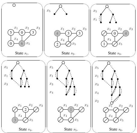
This process is illustrated in Figure 1 for a MISP in-stance. Solid arcs indicate that the vertex related to the cur-rent variable is selected in the solution while dashed arcs indicate the opposite. The partially constructed DD and the inserted/remaining vertices are depicted for each state. The value in each vertex indicates theQˆ-value computed by the

(5)

✬ ✫ ✩ ✪ 5 x1 0 x2 3 x3 0 x4

6 x5

States1.

✬ ✫ ✩ ✪ x5 4 x1 3 x2 3 x3 2 x4 x5

States2.

✬ ✫ ✩ ✪ x5 x1 x1 0 x2 4 x3 1 x4 x5

States3.

✬ ✫ ✩ ✪ x5 x1 x3 x1 2 x2 x3

3 x4

x5

States4.

✬ ✫ ✩ ✪ x5 x1 x3 x4 x1 1 x2 x3

x4

x5

States5.

✬ ✫ ✩ ✪ x5 x1 x3 x4 x2

x1 x2 x3

x4

x5

States6.

Figure 1: Example of an exact DD construction for a MISP instance, following policyπ= argmax_aQπ₍_{s, a}₎_.

Experimental Results

Our first set of experiments are carried out on the MISP, for which the impact of variable ordering has been deeply stud-ied (Bergman et al. 2013). The last experiments analyze the generalization of the approach on the Maximum Cut Prob-lem. For the MISP, the approach is compared with the linear programming relaxation bound, random orderings, and three ordering heuristics commonly used in the literature:

1. Linear Programming Relaxation(LP): The value of the linear relaxation obtained using a standard clique formu-lation for the MISP as described in (Bergman et al. 2013).

2. Random Selection (RAND): An ordering of the vertices is drawn uniformly at random from all permutations. For each test, 100 random trials are performed and the aver-age, best and worst results are reported.

3. Maximal Path Decomposition(MPD): Amaximal path de-compositionis precomputed and used as the ordering of the vertices (Bergman et al. 2013). This ordering bounds the width of the exact DDs by the Fibonacci numbers.

4. Minimum Number of States(MIN): Having constructed up to layerj and hence chosen the firstj −1vertices, the next vertex is selected as the one appearing in the fewest number of states in the DD nodes in layerj. This heuristic aims to minimize greedily the size of the subsequent layer.

5. Minimum Vertex Degree(DEG): The vertices are ordered in ascending order of vertex degree. The vertices with the lowest degree are inserted first.

Experimental Protocol

MISP instances were generated using the Barabasi-Albert (BA) model (Albert and Barab´asi 2002). Such a model is commonly used for generating real-world and scale-free

graphs. They are defined by the number of nodes (n) and an attachment parameter (ν). The greater isν, the denser is the graph. Edges are added preferentially to nodes having a higher degree. Training has been carried out on Compute Canada Cluster1. Training time is limited to 20 hours, mem-ory consumption to 64 GB and one GPU (NVIDIA P100 Pascal, 12GB HBM2 memory) is used. For each configura-tion, the training is done using 1000 generated random BA graphs (between 90 and 100 nodes) that are refreshed ev-ery 5000 iterations. Different models with a specific value for the attachment parameter (ν ={2,4,8,16}) are trained. The model selected is the one giving the best average re-ward on a validation set composed of 100 graphs having the same configuration as the training graphs. The training time required to get this model is dependent on the configuration considered. It varies between 20 minutes for the best case and 6 hours for the worst case. At the first time, testing is carried out on 100 other random graphs of the same size and having the same attachment parameter as for the train-ing. Other configurations are then considered. Performance profiles (Dolan and Mor´e 2002) are used for comparing the approaches. This tool provides a synthetic view on how an approach performs compared to the others tested. The met-ric considered is the optimality gap (i.e. the relative distance between the bound and the optimal solution).

Our model is implemented upon the code of Dai et al.2 for the learning part and upon the code of Bergman et al. (Bergman et al. 2013) for building the DDs of the MISP in-stances. Evaluation of the different orderings is also done using this software. The learning is done using Adam op-timizer (Kingma and Ba 2014). Library networkX (Hag-berg, Swart, and S Chult 2008) is used for generating the random graphs. For the reproducibility of results, the im-plementation of our approach is available online3_{. Optimal} solutions of the MISP instances and the linear relaxations have been obtained using CPLEX 12.6.3.

Results

The goal of the experiments is to show the adequacy of our approach for computing both upper and lower bounds in dif-ferent scenarios commonly considered in practice.

Evaluating the DD Width for Training The first set of experiments aim to determine the best DD maximal width (w) for training the model. Let us first consider ν = 4

for the attachment parameter as in (Khalil et al. 2017). We trained four models (w={2,10,50,100}) for relaxed DDs (RL-UB-4), and tested the models using the same values of

w. Figure 2 shows the performance profiles of the models when evaluated on relaxed DDs of a various width. Random ordering (RAND) is also reported and is outperformed by the four models. The shaded area represent the range of the RANDperformance when considering the best and the worst solution obtained among the 100 trials. Interestingly, these results suggest that the width chosen for the training has a

1_{https://www.computecanada.ca/research-portal/} 2

https://github.com/Hanjun-Dai (graph comb opt)

3

(6)

(a) Testing onw= 2. (b) Testing onw= 10. (c) Testing onw= 50. (d) Testing onw= 100.

Figure 2: Performance profiles of model trained with different widths for relaxed DDs.

(a)ν= 2. (b)ν= 4. (c)ν= 8. (d)ν= 16.

Figure 3: Performance profiles on graphs of different distributions (ν) for relaxed DDs (w= 100).

(a)ν= 2. (b)ν= 4. (c)ν= 8. (d)ν= 16.

Figure 4: Performance profiles on graphs of different distributions (ν) for restricted DDs (w= 2).

negligible impact on the quality of the model, even when the width considered during the testing is different than that for the training. As computing small-width DDs is less com-putationally expensive than those with larger widths, we se-lect the model trained with a width of 2 for the remainder of the experiments on MISP. Concerning restricted DDs, as shown in the next set of experiments (Figures 4a-4d), lower bounds close to the optimal solutions are already obtained with small-width DDs (w = 2). This independence of the width chosen during the training is the most surprising re-sult that we get through our set of experiments. Perhaps one reason of this stability is due to the merging heuristic that remains the same in all the configuration, but an in-depth explanation of these results is still an open question.

Comparison with Other Methods Our approach is now compared to the other variable ordering heuristics using BA graphs having a varied density (ν = {2,4,8,16}). A

(7)

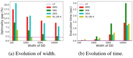
Analysis of Width Evolution Let us now consider the sit-uation depicted in Figure 3b where RL-UB-4 provides a worse bound than the linear relaxation of the problem. Fig-ure 5a depicts the evolution of the optimality gap when the model is tested on relaxed DDs of an increasingly larger width. AsRANDprovided results far outside the range of the other methods for relaxed DDs, we do not include it in the subsequent plots. The plot depicts thatRL-UB-4remains better than the other ordering heuristics tested, and when the DD width is sufficiently large (w > 1000) the LP re-laxation bound is beaten and the optimal solution is almost reached (w= 10000). Figure 5b reports the execution time of the different methods. Concerning the RL model, only the time required for building the DD is reported. We do not re-port the training time on this experiment because it has to be amortized on all the graphs of the test set, which is de-pendent of the situation. The linear relaxation is the fastest method and is almost instantaneous. Concerning the order-ings,RL-UB-4,MPDandDEGare static, and execution time for each generally increases similarly with the width, while MINrequires dynamically processing the nodes in a layer for determining the next vertex to insert.

(a) Evolution of width. (b) Evolution of time.

Figure 5: Relaxed DDs of larger widths (ν = 4).

Analysis of Graph Size Evolution In a similar way, this set of experiments aim to analyze how the learned models perform when larger graphs are considered. Results in Fig-ure 6a depict the optimality gap of the different approaches for relaxed DDs (w= 100).

(a) Relaxed DDs (w= 100). (b) Restricted DDs (w= 2).

Figure 6: Relaxed/Restricted DDs for larger graphs (ν = 4).

We can observe that the learned model remains robust against increases of the graph size although the gap between the other orderings progressively decreases. When the graph

size is far beyond the size used for the training, the model strives to generalize which indicates that training on larger graphs should be required. The LP bounds for large graphs are out of range of DDs of this limited width. The same ex-periment is carried out for restricted DDs and reported in Figure 6b. Given that the optimality is reached even with small-width DDs, only a width of 2 is considered. Here, RL-LB-4provides the best lower bound even for the largest graphs tested. This is consistent with other heuristics imple-mented through RL.

Performance on other Distributions This set of experi-ments aim to analyze the performance of the learned models when they are tested on a different distribution than that used for training. Figure 7 presents the relative gap with the model specifically trained on the distribution tested. For instance, whenν = 8, the gap is computed usingRL-UB-8as ref-erence (or usingRL-LB-8for restricted DDs). We use this measure instead of the optimality gap in order to nullify the impact of the instance difficulty. The gap is then null for the distribution used as reference (RL-UB-4and RL-LB-4). Results show that the more the distribution is distant from the reference, the greater is the gap, which indicates that the learned model strives to generalize. For small perturbations (ν = 2and8), good performances are still achieved. These results suggest that it is important to have clues on the distri-bution of the graphs that we want to access in order to feed appropriately the model during training.

Figure 7: Performance on other distributions.

(8)

higher level of perspective, it empirically shows that an or-dering which is efficient for one situation would not be irre-mediably good for the other one.

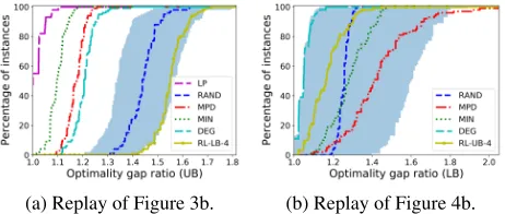
(a) Replay of Figure 3b. (b) Replay of Figure 4b.

Figure 8: Performance of the model trained with restricted DDs on relaxed DDs and inversely.

Experiments on the Maximum Cut Problem

Definition 2 (Maximum Cut Problem) Let G(V, E)be a simple undirected graph. A maximum cut ofGis a subset of nodesI ⊆V such that∑

(u,v)∈Cw(u, v)is maximized,

whereC ⊆ E is the set of edges having a node inS and the other one inV\S. The Maximum Cut Problem (MCP) is that of finding a maximum cut.

As an example of its generalizability, our approach is also applied to the MCP. The DD is built according to formula-tion of (Bergman et al. 2016). The learning process and the model is the same as for the MISP. Generation of graphs is still done using a Barabasi-Albert distribution (ν = 4) with edge weights uniformly and independently generated from

[1,10]. For training, weights are scaled with a factor of 0.01. The ordering obtained is compared withRANDand with the MAX-WEIGHTheuristic which selects the vertex having the highest sum of incoming weights (Bergman et al. 2016). The linear relaxation of a standard integer program of the MCP (Kahruman et al. 2007) is also considered. Results report-ing the optimality gap of the three methods are presented in Figure 9 for relaxed (w= 100for training and testing) and restricted DDs (w= 2).

Figure 9: Performance profiles for the MCP (ν= 4).

In both cases, performances better than RAND and MAX-WEIGHT are reached, indicating that the learn-ing is effective. Concernlearn-ing relaxed DDs, the gap with

MAX-WEIGHT is tighter, which could indicate that this heuristic already gives strong bounds and is then difficult to beat. Finally, the classical linear relaxation does not per-form well on the MCP, which was already known (Avis and Umemoto 2003).

Conclusion

Objective function bounds are paramount to general and scalable algorithms for combinatorial optimization. Deci-sion diagrams provide a novel and flexible mechanism for obtaining high-quality bounds whose output is amenable to improvement through machine learning, since the ob-jective function bound obtained is directly linked to the heuristic choices taken. This paper provides a generic ap-proach based on deep reinforcement learning for finding high-quality heuristics for variable orderings that are shown experimentally to tighten the bounds proven by approxi-mate DDs. Experimental results indicated the promise of the approach when applied to the Maximum Independent Set Problem.

Insights from a thorough experimental evaluation indi-cate: (1) the approach generally outperforms variable or-dering heuristics appearing in the literature; (2) the width chosen during training can have a negligible impact when applied to unseen instances; (3) the model generalizes well when the width is increased and, in most cases, is applied to larger graphs; (4) a separate model must be trained for relaxed and restricted DDs; (5) the approach generalizes to other problems, such as the Maximum Cut Problem; and (6) it is important to have a measure of the distribution on the evaluated graphs in order to be able to feed the model during training. This last point remains a challenge when extending the approach to real-world problems. As a future work, we plan to tackle it by generating new instances for training us-ing generative models from the initial graphs. The idea is to augment the training set by generating new instances, that looks similar in structure to the initial instances, but that are still different.

To the best of our knowledge, this is the first paper to propose the use of machine learning in discrete optimiza-tion algorithms for the purpose of learning both primal and dual bounds in a unified framework. It opens new insights of research and multiple possibilities of future work, such as the application to different domains that utilize DDs as con-straint programming, planning or verification of systems.

References

Albert, R., and Barab´asi, A.-L. 2002. Statistical mechanics of complex networks.Reviews of modern physics74(1):47. Arulkumaran, K.; Deisenroth, M. P.; Brundage, M.; and Bharath, A. A. 2017. A brief survey of deep reinforcement learning.arXiv preprint arXiv:1708.05866.

Avis, D., and Umemoto, J. 2003. Stronger linear program-ming relaxations of max-cut. Mathematical Programming 97(3):451–469.

(9)

Bergman, D.; Cire, A. A.; van Hoeve, W.-J.; and Hooker, J. N. 2012. Variable ordering for the application of BDDs to the maximum independent set problem. InInternational Conference on Integration of Artificial Intelligence (AI) and Operations Research (OR) Techniques in Constraint Pro-gramming, 34–49. Springer.

Bergman, D.; Cire, A. A.; van Hoeve, W.-J.; and Hooker, J. N. 2013. Optimization bounds from binary decision dia-grams. INFORMS Journal on Computing26(2):253–268. Bergman, D.; Cire, A. A.; van Hoeve, W.-J.; and Hooker, J. 2016.Decision diagrams for optimization. Springer.

Bergman, D.; van Hoeve, W.-J.; and Hooker, J. N. 2011. Ma-nipulating MDD relaxations for combinatorial optimization. In Achterberg, T., and Beck, J. C., eds.,Integration of AI and OR Techniques in Constraint Programming for Combi-natorial Optimization Problems, 20–35. Berlin, Heidelberg: Springer Berlin Heidelberg.

Bollig, B., and Wegener, I. 1996. Improving the variable ordering of OBDDs is NP-complete. IEEE Transactions on computers45(9):993–1002.

Bottou, L. 2010. Large-scale machine learning with stochas-tic gradient descent. InProceedings of COMPSTAT’2010. Springer. 177–186.

Bryant, R. E. 1986. Graph-based algorithms for boolean function manipulation. Computers, IEEE Transactions on 100(8):677–691.

Carbin, M. 2006. Learning effective BDD variable orders for BDD-based program analysis.

Dai, H.; Dai, B.; and Song, L. 2016. Discriminative embed-dings of latent variable models for structured data. In Inter-national Conference on Machine Learning, 2702–2711. Deudon, M.; Cournut, P.; Lacoste, A.; Adulyasak, Y.; and Rousseau, L.-M. 2018. Learning heuristics for the TSP by policy gradient. InInternational Conference on the Integra-tion of Constraint Programming, Artificial Intelligence, and Operations Research, 170–181. Springer.

Dolan, E. D., and Mor´e, J. J. 2002. Benchmarking opti-mization software with performance profiles. Mathematical programming91(2):201–213.

Grumberg, O.; Livne, S.; and Markovitch, S. 2011. Learning to order BDD variables in verification. CoRR abs/1107.0020.

Hagberg, A.; Swart, P.; and S Chult, D. 2008. Exploring network structure, dynamics, and function using networkx. Technical report, Los Alamos National Lab.(LANL), Los Alamos, NM (United States).

Henderson, P.; Islam, R.; Bachman, P.; Pineau, J.; Precup, D.; and Meger, D. 2017. Deep reinforcement learning that matters.arXiv preprint arXiv:1709.06560.

Kahruman, S.; Kolotoglu, E.; Butenko, S.; and Hicks, I. V. 2007. On greedy construction heuristics for the MAX-CUT problem. International Journal of Computational Science and Engineering3(3):211–218.

Khalil, E.; Dai, H.; Zhang, Y.; Dilkina, B.; and Song, L. 2017. Learning combinatorial optimization algorithms over

graphs. InAdvances in Neural Information Processing Sys-tems, 6351–6361.

Kingma, D. P., and Ba, J. 2014. Adam: A method for stochastic optimization. arXiv preprint arXiv:1412.6980. LeCun, Y.; Bengio, Y.; and Hinton, G. 2015. Deep learning. nature521(7553):436.

Lee, C.-Y. 1959. Representation of switching circuits by binary-decision programs. Bell system Technical journal 38(4):985–999.

Masters, D., and Luschi, C. 2018. Revisiting small batch training for deep neural networks. arXiv preprint arXiv:1804.07612.

Mnih, V.; Kavukcuoglu, K.; Silver, D.; Graves, A.; Antonoglou, I.; Wierstra, D.; and Riedmiller, M. 2013. Play-ing atari with deep reinforcement learnPlay-ing. arXiv preprint arXiv:1312.5602.

Mnih, V.; Kavukcuoglu, K.; Silver, D.; Rusu, A. A.; Ve-ness, J.; Bellemare, M. G.; Graves, A.; Riedmiller, M.; Fidjeland, A. K.; Ostrovski, G.; et al. 2015. Human-level control through deep reinforcement learning. Nature 518(7540):529.

Riedmiller, M. 2005. Neural fitted Q iteration–first expe-riences with a data efficient neural reinforcement learning method. In European Conference on Machine Learning, 317–328. Springer.

Rumelhart, D. E.; Hinton, G. E.; and Williams, R. J. 1986. Learning representations by back-propagating errors.nature 323(6088):533.

Silver, D.; Huang, A.; Maddison, C. J.; Guez, A.; Sifre, L.; Van Den Driessche, G.; Schrittwieser, J.; Antonoglou, I.; Panneershelvam, V.; Lanctot, M.; et al. 2016. Mastering the game of go with deep neural networks and tree search. nature529(7587):484–489.