by
C.C. OSUAGWU
Department of Electronic Engineering UNIVERSITY OF NIGERIA
NSUKKA
ABSTRACT
A multiplexer with (n-l) data select inputs can realise directly a function of n variables. In this paper, a simple k-map based variable selection scheme is proposed such that an n variable logic function can be synthesised using a multiplexer with (n-q) data input variables and q data select variables. The procedure is based on the fact that if 2X minterms (where x = 1, 2, 3) from a minterm list are adjacent on a k-map, the minimised function read from the map contains information on the variable or variables which form the map highest number of l-cubes. 2-cubes or 3-cubes of the function. Such variables have the lowest frequency of occurrence in the minimised function. The criterion for eliminating (n-q) variables from the data select input is to choose (n-q) variables with the lowest frequencies of occurrence in the minimised function and use them as the data input variables of the multiplexer. The data input values of the multiplexer are obtained by constructing a MEV -map using the (n-q) variables as map entered variables and the q data select variables as mapping variables. The procedure is illustrated with examples.
1.0. INTRODUCTION
The Karnaugh map (k-map) is an invaluable tool in the design of combinational logic circuits using the minimum number of gates. Although advances in integrated circuits have altered the way digital logic design is carried out - (from implementations using the minimum number of gates and external interconnections, to ones using the minimum number of powerful integrated circuit (IC) packages and maximum internal interconnections) - the k-map technique has remained a powerful and systematic tool in the teaching of digital design. The limitations of the k-map is obvious, however. Beyond five variables, the technique becomes very difficult to use and algorithmic approaches like the Quine McCluskey technique become preferable [1].
However, there is no reason for carrying out the synthesis of logic functions of up to six variables using only the primitive AND-OR gates or the more universal NAND or NOR gates. Developments in the subject show that multiplexer-based implementations are ideal for the direct synthesis of such functions using for example, Shannon's expansion theorem (Boolean Algebra) [2] or the map-entered variable (MEV) approach [3, 4, 5]. What has hindered the teaching of multiplexer-based implementations alongside
the traditional gate level implementations in the synthesis of combinational logic functions is probably the lack of a suitable simple manual selection scheme for solving the problem of partitioning the function variables into data select and data input variables. The solution of the partitioning problem is central to the efficient use of multiplexers and those published in the literature result in multiplexer structures with desirable attributes but understandably are designed for computer implementation [6, 7, 8].
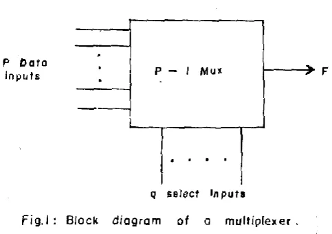
These sought for attributes in the synthesis of logic functions with multiplexers can be stated with the aid of fig 1 as follows:
i) An optimum partitioning of the n variables into q data select and (n-q) data input variables such that the multiplexer input will have a maximum number of logic 1 and logic O connected to it. This minimum input loading criterion of Whitehead [6] implies that (m-2k) data inputs are not connected to logic a and logic 1 where m = umber of minterms in the function and k = number of l-cubes formed by the variable connected to the data input.
that the function is synthesised using the minimum number of multiplexers.
iii) A partitioning of the n variables into q data select and (n-q) data input variables where n > q + 1 which results in an implementation using a single multiplexer without using residue gates Domindo and Canto structure [7].
Osuagwu [9] has shown that the Ashenhurst technique can be used to realise these objectives. But the Ashenhurst technique requires an exhaustive search for all the possible partitions of n variables into q data select variables and (n-q) data input variables in order to select partitions that result in the desired attributes.
In this paper, a simple k-map based variable selection scheme is proposed such that an n variable function can be partitioned into (n-q) data input variables and q data select variables such that the stated attributes are achieved. The technique can be used for functions of up to six variables.
The advantage of the proposed procedure over the algorithmic techniques is that it is a graphical procedure and therefore the exhaustive search for all the l-cubes and 2-cubes of the function is replaced by a simple search using a selection table for the variables with the lowest frequencies of occurrence in the minimised expression. The proposed k-map based variable partition criterion can be sumarised as follows:
1. If the variable with the lowest frequency of occurrence in the minimised expression is used as the map entered variable and the remaining mapping variables used as the data select variables, the Whitehead structure results.
2. If the two variables with the lowest frequency of occurrence in the minimised expression are used as map entered variables and the remaining mapping variables used as the data select variables, the Domindo and Canto structure results, if such a structure exists, otherwise the resulting structure uses residue gates.
3. If the variable that forms the least number of l-cubes of the function is used as the data input variable and the variables with the lowest frequency of occurrence in the minimised function are used as the input multiplexer data select variables; and if the remaining variables are used as the
output multiplexer data select variables, then a minimum tree structure realisation results where such a structure exists. The rest of the paper shows how the criterion was arrived at. Specifically, in section 2, the basis for the k-map variable selection scheme is systematically presented, while section 3 illustrates the procedure with suitable examples.
2.0 K-MAP BASED VARIABLE SELECTION SCHEME
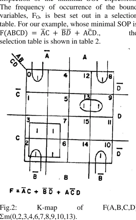
In this section, we show how to use the k-map to partition the function variables into data select and data input variables so as to obtain the prototype multiplexer structures of section 1. We will use the k-map of fig 2 throughout the section to develop the needed theory and illustrate key concepts.
2.1 Definitions O-cube
A O-cube of a logic function consists of the minterm list of the function.
1-cube
Two a-cubes of a function form a l-cube if they differ in only one co-ordinate.
This implies that if two minterms are adjacent on a k-map, they form a 1-cube of the function, for example minterms 9 and 13 in the k-map of fig 2 form the l-cube
̅ ̅̅̅̅ ̅
2-cube.
Four a-cubes of a function form a 2-cube of the function if their co-ordinates are the same except in two variables. From the k-map, the set of four minterms (0,2,8,10) forms the 2-cube ̅ ̅ while (2,3,6,7) forms the 2-cube ̅C.
Bound Components.
The variables of a l-cube or 2-cube for which the co-ordinates are the same are the bound components of the l-cube or 2-cube. For example, in the 2-cube formed by m(0,2,8,10), ̅ ̅ are the bound components.
Free Components.
2.2 Minimum sum of products (SOP) expression.
The minimum sum of products expression for F(A,B,C,D) from the k-map is
̅ ̅ ̅ ̅
The following observations can now be made using the terminologies of section 2.1.:
1. The minimum SOP consists of the essential prime implicants of the function:
m(2,3,6,7); m(0,2,8,10) and m(9,13).
2. The minimum SOP contains only the bound variables of l-cubes, 2-cubes etc.
3. The bound variables carry information about the essential prime implicants and hence about the number of l-cubes of the function formed by each variable of the function. In other words, a relationship exists between the frequency of each bound variable in a minimal SOP and the total number of I-cubes formed by each variable of the function. This relationship is established in section 2.3.
2.3 Relationship between the frequency of each bound variable in a minimal SOP and the total number of I-cubes formed by each of the function.
The need to establish a relationship between the frequency of occurrence of bound
information required to partition the function variables into data select and data input variables in the Whitehead's structure.
ii) the data input variables in the Domindo and Canto structure are chosen from the finite set of variables that form 2-cubes of the function. The key to partitioning the function variables into data select and data input variables in the algorithmic techniques is the determination of the total number of l-cubes formed by each variable of the function as well as the 2-cubes of the function. These information are obtained using the Quine McCluskey technique. This technique is quite laborious and prone to mistakes when used manually. The k-map should be a simple manual way of obtaining the partition information if it can be shown that the frequency of occurrence of bound variables in the minimal SOP can be used to predict the variable that forms the largest number of 1-cubes of the function.
For our running example, the 2-cubes of the function are obvious:
̅̅̅̅̅̅̅̅̅̅̅̅
Table 1:
1 cubes of F(A,B,C,D) = m(0,2,3,4,6,7,8,9,10,13)
Minterm groups A B C D
0/2 8/3 6 9 10/7 13
WA =8 (0,8) (2,10)
WB =4 (2,6) (3,7) (9,13)
WC =2 (0,2) (8,10)
WD =1 (2,3) (8,9) (6,7)
From table 1 we find, by counting the number of minterm pairs under each variable, that the variables B and D form the largest number of 1- cubes of the function.
2.3.1 Frequency of bound variables in a minimal sum of products expression
As we observed in section 2.2, a minimal SOP expression contains only the bound variables of l-cubes, 2-cubes etc. The presence of a bound variable in a SOP expression indicates that variable was not eliminated in the formation of the l-cube of the function. It seems self evident that the higher the frequency of occurrence of a bound variable in a minimal SOP expression, the smaller the total number of l-cubes of the function formed by that variable. Conversely the lower the frequency of occurrence of a bound variable in a minimal SOP expression, the greater the total number of l-cubes of the function formed by that variable. Clearly then, the variable that forms the largest number of 1- cubes of the function will also be the variable with the lowest frequency of occurrence in the minimal SOP expression.
2.3.2 Proof
The easiest way to prove the correctness of these statements is to show that in all cases, the prediction of the variable that forms the greatest number of l-cubes of the function obtained using the Quine McCluskey technique is the same as that obtained by
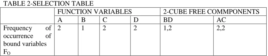
inspection of the minimal SOP expression. The frequency of occurrence of the bound variables, FO, is best set out in a selection table. For our example, whose minimal SOP is
̅ ̅ ̅ ̅ ., the
selection table is shown in table 2.
Fig.2: K-map of F(A,B,C,D)
TABLE 2-SELECTION TABLE
FUNCTION VARIABLES 2-CUBE FREE COMMPONENTS
A B C D BD AC
Frequency of occurrence of bound variables FO
2 1 2 2 1,2 2,2
Since the bound variable A occurs two times in the minimal SOP expression, the value 2 is listed under the function variable A in table 2. The rest of the entries follow. From the selection table, we find that the variable B has the lowest frequency of occurrence in the minimal SOP expression. This implies that it forms the largest number of 1-cubes of the function, a conclusion that agrees with the findings of table 1.
2.3.3 Discussion
It is important to observe that the selection table failed to identify the variable D as forming the largest number of l-cubes also. But this poses no problem since if two or more valid Whitehead's structure exist for the same minterm list, the resulting input loadings in each case are the same. It does not matter, therefore, which of the variables forming the largest number of 1-cubes of the function is selected as the data input variable. In all cases, the selection table will predict accurately the variable that forms the largest number of 1- cubes of a function; and will sift out one or more such variables in situations where two or more variables tie in forming the largest number of 1-cubes of a function.
The selection table (see table 2) also gives the free components of the 2-cubes of the function and associates to each free component the frequency of its bound equivalent from the function variable column. BD has a frequency of (1,2) and this carries the information that the variables Band D together form more 1-cubes of the function than AC with a frequency of (2,2). This prediction agrees with that of table 1 where we find that B and D together form a total of six 1-cubes of the function, while A and C
form a total of four 1-cubes of the function. For the Domindo and Canto structure, the two free component variables which together form the largest number of 1-cubes of the function are used as the data input variables. This is because the resulting residue functions, if the Domindo and Canto structure exists, collapse into logic 1, single input variable or complement of single input variable. It is quite easy to select the data input variables for the Domindo and Canto structure using the selection table. In the present example, we see from the 2-cube free components column of table 2 that BD are the data input variables to choose.
2.4 Connectivity graph
A connectivity graph is a graph that links the free components of the 2-cubes of a function. It shows at a glance the variables which form the free components of the 2-cubes of the function and the variable or variables which do not form any free components in the 2-cubes of the minimised expression. Fig. 3 shows the connectivity graph for our running example.
Notice that all the variables of the function are involved in forming the 2-cubes of the function. Fig. 4 and 5 show the connectivity graphs of the illustrative examples of section 3.
data select variables for the input multiplexers depending on which set has the lowest frequency of occurrence. Since the variables are free components, they will result in multiplexer redundancies and hence give rise to a minimum tree structure realisation
In fig 5 only the variable E is not a free component. This variable should be used as a data input variable in a tree structure implementation in which the data select variables of the input multiplexer consist of the two variables with the lowest frequency of occurrence. The connectivity graph can be used also to identify the free component that is common to as many 2-cubes of the function as possible. The connectivity graph probably carries more information and therefore deserves further study.
2.5 Multiplexer redundancy
Multiplexer redundancy leads to a minimum tree structure realisation.
Now, if a 4-1 multiplexer implements a 2-cube, that multiplexer is redundant since it can always be replaced by the variable or variables corresponding to the bound components of the 2- cube independent of the partition of the function variables into data select and data input variables (8). From our running example, consider the 2- cube m(0,2,8,10) = ̅ ̅. A 4-1 mux implementation of this 2-cube is shown in fig 6 and it is clear the multiplexer implements an AND residue gate.
Let the implementation of fig 6 be equivalently represented by the notation (l, 0, 0, 0): BD
If we use respectively AB, AC, BC, and CD as data select variables to implement this 2-cube, we obtain the following realisations:
̅ ̅ ̅ ̅ ̅ ̅ ̅ ̅ ̅ ̅
̅ ̅ ̅ ̅
̅ ̅
The outputs of these 4-1 multiplexer realisations in each case is ̅ ̅, the bound components of the 2-cube.
The importance of this theorem due to Miller (8) is that if the free components of the 2-cube of a function are used as the data select variables of the input multiplexer, redundancy will result no matter the variable used as the data input variable. In tree structure multiplexer realisation, redundancy is sought in the input multiplexer because the input multiplexer stack contains the largest number of multiplexers
2.6 Summary of procedure
The k-map procedure for partitioning the function variables into data select and data input variables has been presented in this section and is summarised here for ease of reference:
Step 1: Obtain the minimal SOP expression from the k-map of the function.
Step 2: By inspection of the minimised function construct the selection table and the connectivity graph.
Step 3: Determine
i. the variable that forms the largest number of I-cubes of the function ii. the free components with the lowest
frequency of occurrence in the 2-cubes of the function;
iii. the variable or variables that do not form any free components in the 2-cubes of the function
.
Step 4: Depending on the multiplexer structure desired, use the information of step 3 to partition the function variables into data select variables and data input variables
Using the data select variables as the MEV mapping variables and the data input variables as the map entered variables, draw the applicable MEV map. Finally implement the function with multiplexers.
3.0 ILLUSTRATIVE EXAMPLES In this section, we illustrate the procedure with two examples.
3.1 Example 1
Consider the minterm list of:
The k-map, selection table and connectivity graph are shown in figs 7(a), 7(b) and 7(c) respectively.
3.1.1 Elimination of one variable (Whitehead's Structure).
From fig 7(b) we discover that variables A,B, and C have the lowest frequencies of occurrence in the minimised function and will form equal number of 1 cubes of the function (see appendix 1). So any of the three variables can be used as data input variable for a 16-1 mux implementation of the function. The remaining variables will constitute the data select variables. Fig 8 (a) shows the MEV map for the 16-1 mux implementation of the function with A as the data input variable. The resulting multiplexer implementation is denoted equivalently as:
.
3.1.2 Elimination of two variables (Domindo and Canto Structure). For realisation using 8-1 mux, AB, AC or BC can be used as data input variables since these
variables form 2-cubes of the function and have the same frequency of occurrence. The remaining variables constitute the data select variables. Fig 8 (b) shows the MEV map for an 8-1 multiplexer implementation of the function with AB as data input variables and CDE as the data select variables. The resulting multiplexer structure can be denoted equivalently as:
̅ ̅
3.1.3 Elimination of three variables.
From fig 7 (c) we find that the variables DE do not form any free components in the 2-cubes generated by the minimised function. Hence DE must be used as the data select variables for 4-1 mux realisation of the function and the variables A,B,C used as the data input variables. Fig 8 (d) shows the 4-1 mux implementation with ABC as data input variables and DE as the data select variables. Notice the function is realised with a single 4-1 multiplexer without residue gates.
3.2 TREE STRUCTURE
IMPLEMENTATION WITH
horizontally we obtain the tree structure realisation shown in fig 9. This multiplexer realisation can be denoted equivalently as:
Each of the multiplexers labelled 2,3,4 and 5 in fig. 9 implements a 2-cube and is replaced by its bound variable A,O,B,C respectively. The resulting structure is the same as that shown in fig 8(d).
3.2 Example 2
Consider the minterm list
This example illustrates the usefulness of the connectivity graph in identifying a bound variable that can be used as a data input
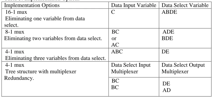
variable so that the function can be realised with a single multiplexer without using residue gates. Fig. 10 shows the k- map of the function while figs. 11 and 12 show respectively the selection table and the connectivity graph. From the function table the variable C forms the largest number of 1-cubes of the function (see also appendix 2). The implementation options are shown in table 3.
16-1 mux implementation
8-1 mux implementation
4-1 mux implementation
Table 3: Implementation Options
Implementation Options Data Input Variable Data Select Variable 16-1 mux
Eliminating one variable from data select.
C ABDE
8-1 mux
Eliminating two variables from data select.
BC or AC
ADE BDE
4-1 mux
Eliminating three variables from data select.
ABC DE
4-1 mux
Tree structure with multiplexer Redundancy.
Data Select Input Multiplexer
Data Select Output Multiplexer
BC
BC DE
̅
Note that the 4-1 mux implementation requires two residue gates.
3.3.1 Tree structure realisation with redundancy
The first tree structure partition in table 3 uses A as data input variable, BC as input multiplexer data select and DE as output multiplexer data select. The applicable MEV map is shown in fig 13.
The resulting tree structure implementation can be equivalently denoted as:
̅ ̅
Notice that the 4-1 multiplexers
implement 2-cubes of the function and are replaced by 0 and 1 respectively. The multiplexer (A,A, 1,1): BC implements the OR residue gate ̅ while the multiplexer (O,O,A,A): BC implements the AND residue gate AB. It is therefore clear that the resulting tree structure realisation shown in fig 14 is equivalent to the 4-1 mux implementation ̅ of table 3.
This implementation uses two residue gates and hence does not result in a Domindo and Canto structure. This data input and data select variable partition was made to obtain the maximum number of logic l's and zeros connected to the data inputs of the multiplexers. Notice that it does not yield the minimum tree structure realisation.
The connectivity graph of fig 5 shows that the variable E is a bound component. Millers theorem guarantees that so long as BC, which form 2-cubes of the function, is used as the input multiplexer-data select, multiplexer
redundancy will result even if the bound variable E is used as the data input variable. We should expect, of course, that the multiplexer inputs will have the minimum number of logic 1 and logic 0 connected to them. This partition, the second tree structure partition in table 3, is discussed in details in section 3.3.2
3.3.2 Second tree structures realisation with redundancy
Here the variable E which forms the least number of 1 cubes of the function is used as the data input variable. This guarantees that the input bus structure will have the minimum number of logic l 's and zeros connected to it. BC is again used as the input multiplexer data select to exploit redundancies that will arise since BC implements 2-cubes of the function The remaining variables AD are used as the data select variables for the output level multiplexer. The applicable MEV map is shown in fig 15. The MEV map of fig 15 is transformed to that of fig 16 so as to orient the variables in the proper mapping order.
Reading the MEV map of fig 16 horizontally, we obtain the multiplexer tree structure realisation denoted equivalently as ̅ ̅ ̅ ̅
The four 4-1 input multiplexers are all redundant since each implements a 2-cube and can be replaced respectively by their bound components:
̅ ̅
implementation without residue gates as follows:
̅ Notice that there is no logic I or logic 0 connected to the multiplexer input.
4. CONCLUSION
A simple k-map based variable selection scheme for partitioning the function variables into q data select and (n-q) data input variables so as to obtain multiplexer implementations with stated optimum attributes has been presented. The ease of use of this manual technique stems from the fact that the variable with the lowest frequency of occurrence in the minimal sum of products expression is also the variable that forms the greatest number of I-cubes of a function. This variable can be selected from an inspection of the minimal sum of products expressed and used as the data input variable of the multiplexer for partitions where n = q + 1.
For partitions where n > q + I. the connectivity graph of the free components of the 2-cubes of a function has been shown to be a useful aid in identifying the bound variable which when used as the data input variable in a tree structure realisation with redundancy, results in a single multiplexer implementation without residue gates. It is hoped that the k-map based variable selection scheme will assist design teachers in the early use of multiplexers in the traditional synthesis of logic functions alongside the more traditional synthesis with universal gates. Multiplexers are afterall universal logic modules and are available.
REFERENCES
1. Hill, F.J., and Peterson, G.R., Introduction to Switching Theory and Logical Design. John Wiley, New York. 1981. Third Edition.
2. Kohavi, Z., Switching Theory and Finite Automata Theory. McGraW-Hill, New York, 1970.
3. Bennett. L. A. M. , The Application of Map-entered Variable to the use of Multiplexers in the Synthesis of Logic Functions". Int. J. Electronics, 1978, Vol. 45, No.4, pp. 373 - 379.
4. Blakeslee. T.R., Digital Design with Standard MSI and LSI. John Wiley, New York, 1975.
5. Fletcher. W.1., An Engineering Approach to Digital Design. Prentice Hall. New Jersey, 1980.
6. Whitehead, D. G., "Algorithm for logic- circuit Synthesis using multiplexers".Electron Lett., 1977. 13, pp. 355 - 256.
7. Dornindo, B., and Canto. D., "Systematic Synthesis of Combinational Circuits using Multiplexers". Electron. Lett., 1978, 14, pp. 588-590.
8. Ektare. A.B., and Mital, A.B., "An Algorithm for Designing Multiplexer Logic Circuits". Int. J. Electronics, 1980, Vol. 49. No.2, pp. 103 - 114.
9. Osuagwu, C.C., "On the use of Ashenhursr Decomposition Chart as an alternative to Algorithmic Techniques in the Synthesis of Multiplexer-Based Logic Circuits". Accepted for publication in Vol. 18 of Nigerian Journal of Technology, NIJOTECH.
10.Li. H. F., "Variable Selection in
Logic Synthesis using
Multiplexers". Int. J. Electronics, 1980, Vol. 19. No.3, pp. 185 - 195.
APPENDIX 1
Minterms arranged in Groups according to the number of one's in their binary representation G1 = (2,16); G2 = (6,18,20,24); G3 = (7,22,28); G4 = (15,23); G5 = 31
A B C D E
WA= 16 WB = 8 We = 4 WD = 2 WE = 1
(2,18) (16,24) (2,6) (16,18) (6,7)
(6,22) (20,28) ( 16,20) (20,22) (22,23)
(7,23) (7,15) (18,22)
(15,31 ) (23,31) (24,28)
1-cubes of minterm list of Example 3-1 showing that variables A, B and C tie in forming the largest number of 1-cubes of the function.
APPENDIX 2
Minterms arranged in Groups according to the number of one's in their binary representation.
G1 = (1,2); G2 = (5,6,9,10,17); G3 = (13,14,21,25,26); G4 = (27,29,30); G5 = 31.
A B C D E
WA = 16 WB = 8 We = 4 WD = 2 WE= 1
(1,17) (1,9) (1,5) (25,27) (26,27)
(5,21 ) (2,10) (9,13) (29,31) (30,31)
(9,25) (2,13) (10,14) (10,26
)
(6,14) (17,21) (13,29
)
(17,25) (25,29) (14,30
)
(21,29) (26,30) (27 ,31)