A New Class of Decentralized Interaction Estimators for Load Frequency Control in Multi-Area Power Systems

(1)

A NEW CLASS OF DECENTRALIZED INTERACTION

ESTIMATORS FOR LOAD FREQUENCY CONTROL

IN MULTI-AREA POWER SYSTEMS

M. H. Kazemi

Department of Electrical Engineering, Shahed University Tehran, Iran, [email protected]

M. Karrari and M. B. Menhaj

Department of Electrical Engineering, Amirkabir University Tehran, Iran, [email protected] - [email protected]

(Received: March 25, 2001 – Accepted: December 12, 2002)

Abstract Load Frequency Control (LFC) has received considerable attention during last decades.

This paper proposes a new method for designing decentralized interaction estimators for interconnected large-scale systems and utilizes it to multi-area power systems. For each local area, a local estimator is designed to estimate the interactions of this area using only the local output measurements. In fact, these interactions are the information of other area. A new scheme is developed to construct an approximate model for the interaction dynamics and design a local estimator. The designed local estimator exploits the model of each area and its actual inputs and outputs to produce a good estimation of unknown states and interactions. It is shown that in the proposed method the errors of estimation are globally ultimately bounded with respect to a specific bound. Our scheme is used to design decentralized estimator for a three-area power system to illustrate the effectiveness of the proposed method.

Key Words Multi Area Power System, Load Frequency Control, Large Scale Systems, Estimation

ﻩﺪﻴﮑﭼ

ﺭﺎﺑ ﻝﺮﺘﻨﮐﺮﻴﺧﺍ ﻪﻫﺩﺭﺩ

ﺲﻧﺎﮐﺮﻓ ) LFC (

ﺖﺳﺍ ﻪﺘﻓﺮﮔ ﺭﺍﺮﻗﯼﺩﺎﻳﺯﻪﺟﻮﺗ ﺩﺭﻮﻣ .

ﺵﻭﺭﻪﻟﺎﻘﻣﻦﻳﺍ ﺭﺩ

ﻱﺪﻳﺪﺟ ﻱﺍﺮﺑ

ﺑﺍ ﻱﺎﻬﻤﺘﺴﻴﺳﻲﻠﺧﺍﺪﺗ ﺕﺍﺮﺛﺍﺰﮐﺮﻤﺘﻣ ﺎﻧﻦﻴﻤﺨﺗ ﺕﺭﺪﻗﻢﺘﺴﻴﺳ ﮏﻳﺭﺩﻥﺁ ﻱﺮﻴﮔﺭﺎﮑﺑ ﻭﻊﻴﺳﻭ ﺩﺎﻌ

ﻲﻣﻪﺋﺍﺭﺍﻱﺍﻪﻴﺣﺎﻧﺪﻨﭼ ﺩﺩﺮﮔ

.

ﻴﻠﺤﻣﺮﮕﻨﻴﻤﺨﺗﮏﻳ ﻪ

ﻱﺍﺮﺑ ﻲﺣﺍﺮﻃﻲﻠﺤﻣﻪﻴﺣﺎﻧﺮﻫﻪﺑﻩﺩﺭﺍﻭﻲﻠﺧﺍﺪﺗﺕﺍﺮﺛﺍﻦﻴﻤﺨﺗ

ﻲﻣ ﺩﺩﺮﮔ .

ﻲﻠﺧﺍﺪﺗﺕﺍﺮﺛﺍﻦﻳﺍ ،

ﻲﻣﻲﺣﺍﻮﻧﺮﻳﺎﺳﺯﺍﻲﺗﺎﻋﻼﻃﺍ،ﺖﻘﻴﻘﺣﺭﺩ ﺪﻨﺷﺎﺑ

. ﻲﺒﻳﺮﻘﺗﻲﻟﺪﻣ،ﺪﻳﺪﺟﺵﻭﺭﮏﻳﻲﻃ

ﺍﺪﺗ ﺕﺍﺮﺛﺍﮏﻴﻣﺎﻨﻳﺩﺯﺍ

ﻲﻣﻪﺘﺧﺎﺳﻲﻠﺧ

ﻲﻣﻲﺣﺍﺮﻃﻲﻠﺤﻣﺮﮕﻨﻴﻤﺨﺗ ﻭﺩﻮﺷ ﺩﺩﺮﮔ

. ﺯﺍﻩﺩﺎﻔﺘﺳﺍﺎﺑﻪﻴﺣﺎﻧﺮﻫﺮﮕﻨﻴﻤﺨﺗ

ﻲﻣﺖﺳﺪﺑﺍﺭﻪﺘﺧﺎﻨﺷﺎﻧﺖﻟﺎﺣﯼﺎﻫﺮﻴﻐﺘﻣﻭﻲﻠﺧﺍﺪﺗﺕﺍﺮﺛﺍﺯﺍﻲﻨﻴﻤﺨﺗ،ﻪﻴﺣﺎﻧﻥﺁﯼﺎﻫﻲﺟﻭﺮﺧﻭﺎﻫﻱﺩﻭﺭﻭ ﺩﺭﻭﺁ

.

ﺍﺮﮕﻤﻫﺺﺨﺸﻣﻩﺩﻭﺪﺤﻣﮏﻳﻪﺑﻲﻳﺎﻬﻧﺭﻮﻃﻪﺑﻦﻴﻤﺨﺗﯼﺎﻄﺧﻪﮐﺖﺳﺍﻩﺪﺷﻩﺩﺍﺩﻥﺎﺸﻧ،ﻪﻴﻀﻗﺪﻨﭼﻲﻃ ﻲﻣ

ﺩﺩﺮﮔ .

ﻱﺍﺮﺑ ﻱﺩﺎﻬﻨﺸﻴﭘﺵﻭﺭ،ﺮﺘﺸﻴﺑﯼﺎﻫﺖﻴﻠﺑﺎﻗﻥﺩﺍﺩﻥﺎﺸﻧ ﺭﻮﻈﻨﻣﻪﺑ

ﺎﻧﺮﮕﻨﻴﻤﺨﺗﻲﺣﺍﺮﻃ ﺕﺭﺪﻗﻢﺘﺴﻴﺳﮏﻳﺭﺩﺰﮐﺮﻤﺘﻣ

ﺖﺳﺍﻩﺪﻳﺩﺮﮔﯼﺯﺎﺳﻩﺩﺎﻴﭘﯼﺍﻪﻴﺣﺎﻧﻪﺳ .

1. INTRODUCTION

In Power systems, one of the most important issues is load frequency control (LFC), which deals with the problem of how to deliver the demanded power at the desired frequency with minimum transient oscillations [1]. This problem has received considerable attentions during the last three decades led to development of many different approaches [2-4]. Load frequency control in a multi-area power system is an example of large-scale systems, which

(2)

yields the better results.

The classical scheme for decentralized state feedback control is based on the assumption that all states of the subsystems are available [10-11]. In large-scale systems, especially multi-area power systems, however, this assumption is not usually realistic. Therefore, a state estimator has to be designed. This estimator exploits the model of each subsystem and its actual inputs and outputs to produce a good estimation of unknown states of the system. Interactions between subsystems are another uncertainties that make the complexity of controller design in large-scale systems. In the classical scheme for decentralized control, the interactions are unknown for the local observer or controller. Therefore the reconstruction of interactions plays an important role in the local observers and controllers to achieve less conservative performance. The main idea of this paper is to introduce a scheme to estimate the interactions in a decentralized approach. The decentralized observation problem was first considered in [12]. Necessary and sufficient conditions on the subsystems were derived in [13] under which the observers could be designed. In [14] an output-decentralization and stabilization scheme were proposed, which could be directly used to construct asymptotic state estimators for linear large-scale systems. The problem of robustness of a Luenberger observer applied to a given large-scale system was addressed in [15].

In [16] a decentralized filter was obtained by identifying the dynamics of the interaction variables, and estimating the local states and interactions using local information. An indirect method for decentralized estimation of interconnected large-scale systems was presented in [17]. In [17], the estimators were obtained in two steps. In the first step, an approximate model for the desired local variables, in an indirect method, was derived. In the second step a local filter was derived using the obtained model and the local measurements. In the previously published papers, [16-19], either the local state vector and the interaction variables are assumed to be available or the interactions have been treated as disturbances. However in the practical problems, as considered in this paper, there is no measurement on the interaction variables. Our main objective, in this paper, is to introduce a new method for designing decentralized estimators

to estimate the states and interactions, using only local output feedback.

In a decentralized control problem, such as decentralized state estimation or the interaction estimation problem, the overall large-scale system is split into the two systems, the related subsystem (ith subsystem) and the residue system (aggregation of other subsystems). It should be noted that, the interactions to the ith subsystem are generated by the dynamics of the residue system. Therefore, by incorporating the dynamics of the residue system one can expect to reduce the error of the estimation. Now, if the dynamics of the residue system is added to the estimator dynamics, the order of the designed filter becomes very high, while, the aim of decentralized estimation is to use low order estimator for each subsystem.

This paper is organized as follows: Section 2 formulates the problem. The system under study is described in Section 3. Section 4 is devoted to present the main contributions of this paper namely as: (1) introducing a new technique for interaction dynamics identification and (2) developing a new decentralized states and interactions estimator, which uses the identified model. In Section 5, the simulation results for a three-area power system show the effectiveness of the proposed algorithm.

2. PROBLEM STATEMENT

Consider the large-scale LTI system S, composed of N subsystem S_i (

i

=

1

,

2

,...,

N

) described by

i i i i

i i i i i i ii i

v

x

C

y

w

G

u

B

h

x

A

x

+

=

+

=

&

(1)

where,

h

_i is the interaction from other subsystems,

∑

≠ =

=

N

i j1 j

j ij

i

A

x

h

(2)

where ni

i

R

x

∈

is the state vector of ith subsystem and pi

i

R

u

∈

is its control function. Furthermore i

g

i

R

w

∈

is the disturbance and qi i R

(3)

measurement noise, which is assumed be bounded

ii

A

,

B

_i,

C

_i, and

G

_i describe the dynamics of the isolated ith subsystem,

A

_ij describes the interaction matrix from the jth subsystem, which are assumed to have appropriate dimensions. It is assumed that

(

C

i

,

A

ii

)

is observable and

(

A

ii

,

B

i

)

is controllable.

The goal of this paper is to design an estimator

i

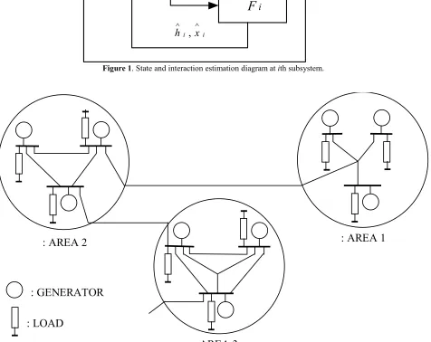
F for each subsystem to estimate the interactions from other subsystems, h_i, and the states of ith subsystem. As seen in Figure 1, the estimator F_i

L o c a l

C o n tr o ll e r

O th e r

S u b s y s te m s

S

i

F

i

h

i

x

i

∧ ∧

,

u

i

y

i

v

i

w

i

h

i

x

i

R e f.

Figure 1. State and interaction estimation diagram at ith subsystem.

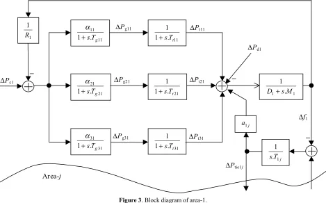
: LOAD

: GENERATOR

: AREA 2

: AREA 3

: AREA 1

(4)

constructs the estimate of interaction, hˆ_i, and state estimation

xˆ

_i from the input and output of

S

_i. The local controller uses these estimations to control the ith subsystem.

3. THE SYSTEM UNDER STUDY

A three-area power system shown in Figure 2 is taken as an example system [20].

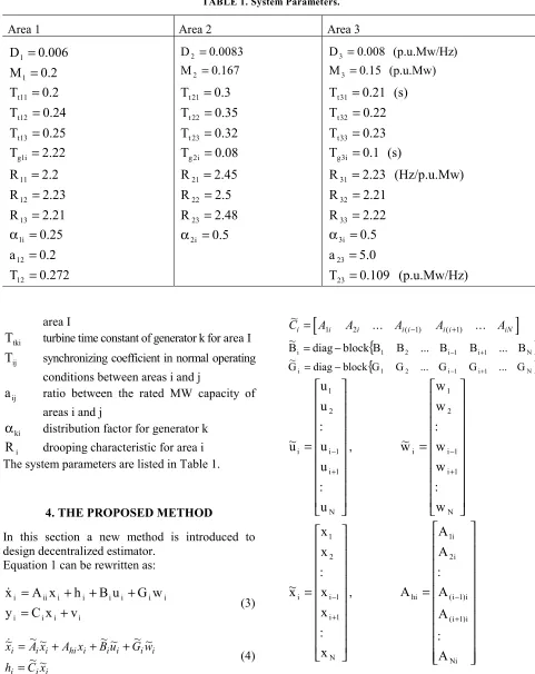
Figure 3 shows the block diagram of area 1. Referring to Figure 3, state vector x, control vector u, and disturbance vector d can be defined as follows:













=

3 2 1

x

,













∆

=

3 c

2 c

1 c

P

u

,













∆

=

3 d

2 d

1 d

P

d

,













=

3 2 1

y

[

f

P

]

T

y

₁

=

∆

₁

∆

_tie₁₂ ,

y

₂

=

[

∆

f

₂

∆

P

_tie₂₃

]

T

,

[ ]

f

T

y

₃

=

∆

₃

[

_f _P _P _P _P _P _P _P

]

T

x1= ∆1 ∆ t11 ∆ t21 ∆ t31 ∆ g11 ∆ g21 ∆ g31 ∆ tie12

[

_f _P _P _P _P _P _P _P

]

T

x2=∆ 2 ∆ t12 ∆ t22 ∆ t32 ∆ gt12 ∆ g22 ∆ g32 ∆ tie23

[

]

T

33 g 23 g 13 g 33 t 23 t 13 t 3

3 f P P P P P P

x = ∆ ∆ ∆ ∆ ∆ ∆ ∆

where,

i

f

∆ incremental frequency deviation of area I

gki

P

∆

incremental governor valve position change of generator k of area I

ci

P

∆

control input of area I

tki

P

∆

incremental output of generator k in area I

ij tie

P

∆

incremental change in tie-line power between areas i and j

di

P

∆

disturbance of area I

i

M

equivalent inertia constant for area I

i

D

equivalent damping coefficient for area I

gki

T

governor time constant of generator k for

11 11 . 1+sT_g

α

11 . 1

1

t

T s

+

1

1 .

1 M s

D +

21 21 . 1₊sT_g

α

21 . 1

1

t

T s

+

31 31 . 1+sT_g

α

31 . 1

1

t

T s

+

j

T s. 1

1

j

a1

∆Pc1

∆Pg11

∆Pg21

∆Pg31

∆Pt11

∆Pt21

∆Pt31

∆Ptie1j

1 1 R

∆Pd1

∆f1

Area-j

(5)

area I

tki

T

turbine time constant of generator k for area I

ij

T

synchronizing coefficient in normal operating conditions between areas i and j

ij

a

ratio between the rated MW capacity of areas i and j

ki

α

distribution factor for generator k

i

R

drooping characteristic for area i The system parameters are listed in Table 1.

4. THE PROPOSED METHOD

In this section a new method is introduced to design decentralized estimator.

Equation 1 can be rewritten as:

i i i i i i i i i i ii i

v

x

C

y

w

G

u

B

h

x

A

x

+

=

+

=

&

(3) i i i i i i i i hi i i i x C h w G u B x A x A x ~ ~ ~ ~ ~ ~ ~ ~ ~ = + + + = & (4) where,

[

]

~ _... _... ( ) ( )

C_i ₌ A₁_i A₂_i A_{i i}₋₁ A_{i i}₊₁ A_iN

{

1 2 i1 i1 N

}

i diag blockB B ... B B ... B

B~ = − ₋ ₊

{

1 2 i 1 i 1 N

}

i diag block G G ... G G ... G

G~ = − − +













=

+ − N 1 i 1 i 2 1 i

u

:

u

:

u

u~

,













=

+ − N 1 i 1 i 2 1 i

w

:

w

:

w

~













=

+ − N 1 i 1 i 2 1 i

x

:

x

:

x

x~

,













=

+ − Ni i ) 1 i ( i ) 1 i ( i 2 i 1 hi

A

:

A

:

A

For convenience, in Part A of this section, the overall system dynamics is considered without TABLE 1. System Parameters.

Area 1 Area 2 Area 3

2

.

0

M

006

.

0

D

1 1

=

167 . 0 M 0083 . 0 D 2 2 = = (p.u.Mw) 15 . 0 M ) (p.u.Mw/Hz 008 . 0 D 3 3 = =

25

.

0

T

24

.

0

T

2

.

0

T

13 t 12 t 11 t

=

32

.

0

T

35

.

0

T

3

.

0

T

23 t 22 t 21 t

=

23

.

0

T

22

.

0

T

(s)

21

.

0

T

33 t 32 t 31 t

=

21

.

2

R

23

.

2

R

2

.

2

R

22

.

2

T

13 12 11 i 1 g

=

48

.

2

R

5

.

2

R

45

.

2

R

08

.

0

T

23 22 21 i 2 g

=

22

.

2

R

21

.

2

R

)

(Hz/p.u.Mw

23

.

2

R

(s)

1

.

0

T

33 32 31 i 3 g

=

272

.

0

T

2

.

0

a

25

.

0

12 12 i 1

=

α

₂_i

=

0

.

5

(6)

any control inputs, measurement noise, and disturbances. In Part B, the results are extended to the general case where all of these assumptions are relaxed.                       = + − + + + − + + + − + − − − − − + − + − NN ) 1 i ( N ) 1 i ( N 2 N 1 N N ) 1 i ( ) 1 i )( 1 i ( ) 1 i )( 1 i ( 2 ) 1 i ( 1 ) 1 i ( N ) 1 i ( ) 1 i )( 1 i ( ) 1 i )( 1 i ( 2 ) 1 i ( 1 ) 1 i ( N 2 ) 1 i ( 2 ) 1 i ( 2 22 21 N 1 ) 1 i ( 1 ) 1 i ( 1 12 11 i A ... A A ... A A : : : : : : : A ... A A ... A A A ... A A ... A A : : : : : : : A ... A A ... A A A ... A A ... A A A~

A. The Simplified Case

Consider the dynamics models 3 and 4, without any control inputs, measurement noise, and disturbances, i.e.,

i i ii

i

A

x

h

x

&

=

+

i hi i i

i

A

x~

A

x

~

x~

&

=

+

i i

i

C

x~

~

h

=

i i i

i

C

x

v

y

=

+

(5) Now let’s define the following estimator:

(

i i i

)

1 i i ii

i

A

xˆ

hˆ

K

y

C

xˆ

&

=

+

−

(

i i i

)

2 i i

i

=

M

ξ

+

N

xˆ

+

K

y

−

C

xˆ

ξ

&

i

E

hˆ

=

ξ

(6) where,

K

₁ and

K

₂are filter gains and E, M, N, are

appropriately dimensioned design matrices which substitute for the dynamics of the interactions.

ξ

_i is a state variable vector, which is considered for dynamics of the interactions. Let us set the dimension of

ξ

_i equal to the dimension of

x

_i. Now, the appropriate values of E, M, N should be found such that the best response for the estimator 6 and bounded error estimation are achieved.

Let the estimation errors be defined as:

i i

x

xˆ

e

=

−

i i

h

hˆ

e

=

−

(7)

where,

e

_x is the error of state estimation and

e

_h is the error of interaction estimation. Then for the state error, we have:

(

ii 1 i

)

x h

i i 1 i 1 i i ii i i i ii i i x e e C K A xˆ C K y K E xˆ A x~ C~ x A xˆ x e + − = + − ξ − − + = − = & & &

(8) and for the interaction error, we have:

(

)

(

i hi i i

)

i i i i 2 i x i i i 2 i i i hi i i i i i i i i i h e C EK EM x~ A~ C~ xˆ EN x A C~ xˆ C y EK EM xˆ EN x A C ~ x~ A~ C ~ = . E x~ C~ hˆ h e − ξ − + − = − − ξ − − + ξ − = −

=& & & &

(9) Now let’s choose the matrices E and N such

that,

hi i

A

C

~

EN

=

(10)

then, Equation 9 can be rewrite as:

(

i hi 2 i

)

x i i i i

h

A

x~

EM

~

C

~

e

C

EK

A

C

~

e

&

=

−

+

−

ξ

(11) Assuming that E is nonsingular, the above equation

can be written in the form:

(

i hi 2 i

)

x 1 h

(

i i 1 i

)

i

h C x~

~ EME A~ C~ e EME e C EK A C~

e_& ₌ ₋ ₊ − ₊ ₋ −

(12) Augmenting 8 with 12, the error equation can be

written as: i i 1 i i h x 1 i 2 hi i i 1 ii h x _x~ C~ EME A~ C ~ 0 e e EME C EK A C~ I C K A e e       − +             − − =       − − & & (13) By defining:













−

=

₋₁

i 2 hi i i 1 ii

EME

C

EK

A

C

~

I

C

K

A

:

H

,













=

h x

e

,













−

=

₋ i 1 i i

C

~

EME

A

~

C

~

0

(7)

the Equation 13 become:

i

x~

F

He

e

&

=

+

(15)

Theorem 1

The solutions

e

(

t

;

t

₀

,

e

₀

)

of the error system 13 are globally ultimately bounded with respect to a bound

V

_f if H is chosen as a stable matrix and

x~

_i are bounded.

Proof Let’s choose H as a stable matrix such that for any symmetric positive definite matrix Q there exists a unique symmetric positive definite matrix P as the solution of the Lyapunov matrix equation:

Q

PH

P

H

T

+

=

−

₍₁₆₎

Then we define a function

V

:

R

2ni

→

R

+_as:

( )

e

Pe

V

=

γ

T ₍₁₇₎

where,

γ

is a positive number. Computing

V

&

( )

e

using 15, results in:

( )

e

(

H

P

PH

)

e

2

x~

F

Pe

V

T

i T

T

+

γ

=

&

,

( )

t

,

e

∈

R

×

R

2ni

∀

(18) now using 16, we have:

( )

e

Qe

2

x~

F

Pe

V

T

i

T

+

γ

−

=

&

,

∀

( )

t

,

e

∈

R

×

R

2ni

(19)

and then the term

x~

F

T

Pe

i

γ

can be written as:

( )

(

) (

)

e

P

e

x~

F

x~

Pe

x~

F

Pe

x~

F

Qe

e

V

2 T 2 i T T i

i T i

T

γ

+

γ

−

γ

−

γ

−

=

&

( )

t

,

e

∈

R

×

R

2ni

∀

(20) by dropping some negative terms and using the

bounded ness assumption of

x~

_i, the following inequality is obtained:

( )

(

( )

2

)

2

min 2

F

P

Q

e

V

&

≤

γ

−

λ

+

γ

+

χ

( )

t

,

e

∈

R

×

R

2ni

∀

(21)

where,

( )

2 i t

t

x~

sup

=

χ

(22)

The last inequality can be summarized as:

( )

e

≤

−

ζ

e

2

+

η

V

&

,

∀

( )

t

,

e

∈

R

×

R

2ni (23)

where, the constants

ζ

and

η

are defined to be:

( )

[

λ

−

γ

]

γ

=

ζ

min

Q

P

2 ,

2

F

χ

=

η

(24)

Selecting

γ

*small enough such that

ζ

>

0

, then 23 implies:

( )

e

≤

−

µ

V

( )

e

+

η

V

&

,

∀

( )

t

,

e

∈

R

×

R

2ni (25)

where, the positive number

µ

is given by

( )

P

1 max

1 −

−

λ

ζγ

≤

µ

(26)

From 25 it is clear that

V

(

e

)

decreases monotonically along any solution of 23 until the solution reaches the compact set:

( )

{

2ni f

}

f

=

e

∈

R

:

V

e

≤

V

Ω

(27)

where,

η

µ

=

−1 f

V

(28)

Therefore the solutions

e

(

t

;

t

₀

,

e

₀

)

of 13 are globally ultimately stable with respect to bound

f

V

. Q.E.D

From 15 it is clear that if

F

=

0

and H is stable, the error e converges to zero. To choose the matrices M, N, E, the first step is satisfying the stability condition of matrix H.

The following Lemma gives the stability condition of matrix H.

(8)

Condition 1: The couple (

A

_H

,

C

_H) be observable,

where,

,

C

[

C

0

]

EME

A

C

~

I

A

₁ _H _i

hi i

ii

H



=











=

₋

then we can stabilize the matrix H by selecting the appropriate filter gains.

Proof

From 14 we can rewrite the matrix H as the form

H H

H

K

C

A

H

=

−

(29)

where,













=

2 1

H

EK

K

Therefore, if the observability condition of (

A

_H

,

C

_H) is satisfied, then there exists a gain

K

_H such that H is stable. Note that we can compute the gain matrix

K

_H as a LQE problem for the system (

A

_H

,

C

_H) such as previous sections. Q.E.D

Selection of E and N

It seems that there are some degrees of freedom for the selection of the matrix E, but according to Theorem 3.1, first the effect of matrix E on the upper bound of the error estimation and the possibility of decreasing it should be investigated.

Equations 28, 26, and 24, imply that:

( )

2

min max 1

f

P

Q

P

V

γ

−

λ

≤

η

µ

=

− ₍₃₀₎

From 30, it can be noted that the larger Q and lower P, results in decreasing the upper bound

V

_f . For a fixed matrix Q, increasing the matrix H results in small P matrix, i.e., the unique solution of the Lyapunov matrix Equation 16. Therefore the matrix H should be high, by appropriate selection of E.

If the matrix E is chosen as:

I

E

=

ρ

(31)

then, by increasing _ρ, the element

(

2

×

1

)

of the matrix H become high. The precise value of _ρ can only be obtained by trial and error.

From 10 and 31, the matrix N can be get as:

hi i 1

C

~

A

N

=

ρ

− ₍₃₂₎

Selection of M

As stated in the previous section, if

F

=

0

and H is stable then the error e converges to zero. Unfortunately as seen in 14) F cannot always be equal to zero, because, the matrix

C

~

_i

may be not a full rank matrix. But we can choose the matrix M such the effect of F is minimized. In the other word, M can be achieved from the following optimization problem:

3.1

condition

S.t

C

~

M

A

~

C

~

M

min

F

M

min

=

_i _i

−

_i

(33)

One solution of 33 in the absence of condition 3.1 is

⊥

=

i i

C

i

~

A

~

C

~

M

(34)

where,

C

~

⊥_i is the pseudo-inverse of

C

~

_i.

Therefore by using 31, 32, 34 and Lemma 2, the estimator 6 can be constructed.

B. The General Case

Now, the above method is extended to the general case, when the input disturbance, measurement noise, and external input are present. Hence consider the large-scale system which is introduced by Equations 3,4, and the following estimator can be defined:

(

i i i

)

i i 1

i i ii

i

A

xˆ

hˆ

K

y

C

xˆ

B

u

xˆ

&

=

+

−

+

(

i i i

)

2 i i

i

=

M

ξ

+

N

xˆ

+

K

y

−

C

xˆ

ξ

&

i

E

hˆ

=

ξ

i i i

i

C

x

v

y

=

+

(35) Let the error of estimation be defined as 7, and as a

result the error system dynamics as:

(

)



  

 

+ +

− −

−

+          

 

− − =

     

−

i i i i i i i 2 i i 1 i

i

i 1 i i

h x 1 i

2 hi i

i 1 ii

h x

w~ G~ C ~ u~ B~ C~ v EK x~ C~ EME A~

C~

v K w G

e e EME C

EK A C~

I C

K A e

e & &

(9)

2 12

1(8) T f

h = ∆

0 1 2 3 4 5 6 7 8 9 10

-0.2 -0.15 -0.1 -0.05 0 0.05 0.1 0.15

Time

:Actual :Estimate

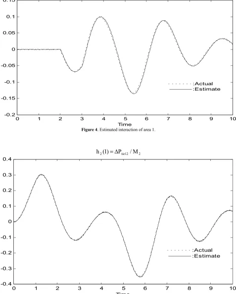
Figure 4. Estimated interaction of area 1.

2 12 tie

2

(

1

)

P

/

M

h

=

∆

0 1 2 3 4 5 6 7 8 9 10

-0.4 -0.3 -0.2 -0.1 0 0.1 0.2 0.3 0.4

Time

:Actual :Estimate

(10)

3 23

2(8) T f

h = ∆

0 1 2 3 4 5 6 7 8 9 10

-0.04 -0.03 -0.02 -0.01 0 0.01 0.02

Time

:Actual :Estimate

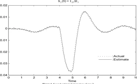
Figure 6. Second estimated interaction of area 2.

3 23 tie

3

(

1

)

P

/

M

h

=

∆

0 1 2 3 4 5 6 7 8 9 10

-0.1 -0.05 0 0.05 0.1 0.15 0.2 0.25

Time

:Actual :Estimate

(11)

By defining H and e as 14 and f as:

(

)

_

  

+ +

− −

−

= ₋

i i i i i i i 2 i i 1 i

i

i 1 i i

w~ G~ C~ u~ B~ C~ v EK x~ C~ EME A~

C~

v K w G :

f

(37) the error system 36 can be summarized to:

f He

e& = + (38)

Theorem 2

The solutions

e

(

t

;

t

₀

,

e

₀

)

of the error system 36 are globally ultimately bounded with respect to a bound

V

_f if H is chosen as a stable

matrix and

x~

_i,

w

~

_i,

u~

_i be bounded signals.

Proof

Similar to proofs of Theorem 3.1 we define a function

V

:

R

2ni

→

R

+_{as 17 and compute}

( )

e

V

&

with respect to 38 and using 16, we have,

( )

e e Qe

(

f Pe

) (

f Pe

)

f f e P e

V_& ₌₋_γ T ₋ ₋_γ T ₋_γ ₊ T ₊_γ2 T 2

,

∀

( )

t

,

e

∈

R

×

R

2ni

(39) By dropping some negative terms and using the

boundedness assumption of

x~

_i,

w

~

_i,

u~

_i, which means the boundedness of f, the following inequality is obtained.

( )

e

≤

−

ζ

e

2

+

η

V

&

, _∀

( )

t e, _{∈ ×}R R2ni (40)

where,

( )

2 t

t

f

sup

=

η

,

ζ

=

[

λ

_min

( )

Q

−

P

2

γ

]

γ

(41)

Selecting

γ

*_{small enough so that}

ζ

>

₀

_{, Equation}

40 implies:

( )

e

≤

−

µ

V

( )

e

+

η

V

&

,

∀

( )

t

,

e

∈

R

×

R

2ni (42)

where, the positive number 1

( )

P

max

1 −

−

λ

ζγ

≤

µ

is

given as 26.

From 42) it is clear that

V

(

e

)

decreases monotonically along any solution of 36 until the solution reaches the compact set

( )

{

2ni f

}

f

=

e

∈

R

:

V

e

≤

V

Ω

,

=

µ

−1

η

f

V

(43)

Therefore the solutions

e

(

t

;

t

₀

,

e

₀

)

of 36 are globally ultimately stable with respect to bound

f

V

. Q.E.D

Hence, the same results in Part A for selection of matrices M, N, E, are valid.

5. SIMULATION RESULTS

In order to demonstrate the effectiveness of the proposed decentralized interaction estimation, numerical simulations have been carried out. Now

3 23 tie

3

(

1

)

P

/

M

h

=

∆

0 1 2 3 4 5 6 7 8 9 10

-0.1 -0.05 0 0.05 0.1 0.15 0.2 0.25

Time

ρ = 10 ρ = 20 ρ = 50 ρ = 100

Actual

Figure 8. Estimated interaction of area 3 for some different ρ.

3 23 tie

3

(

1

)

P

/

M

h

=

∆

0 1 2 3 4 5 6 7 8 9 10

-0.1 -0.05 0 0.05 0.1 0.15 0.2 0.25

Time

(12)

the proposed interaction estimation method is implemented to a multi-area power system, which is described in Section 3. For each area, it is assumed that there occurs 0.1 puMW step disturbance in other two area and also there is 0.01 percent measurement noise. A local estimator is design for

100

=

ρ

at each area and the estimated interactions are shown in Figures 4 to 7. Figures 8 shows the real and estimated interactions of area 3 for

ρ

=10, 20,50, and 100. As we can see from this figure, we may still improve the estimator behavior by increasing the parameter

ρ

. More increasing of _ρ caused the noisy results, as shown in Figure 9 for

ρ

=1000. The precise value of this parameter (

ρ

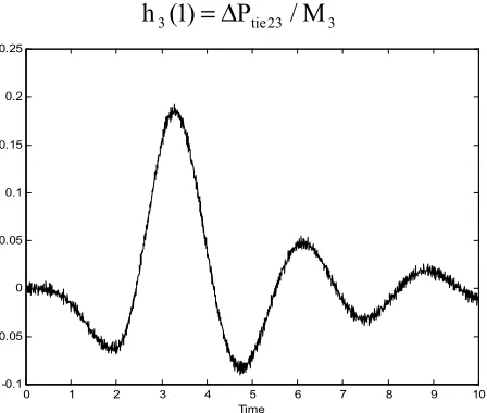
) can be obtained by trial and error.

It should be noted that, since the estimation of interactions is the main goal of this paper, no control input signals,

∆

P

_ci, are considered for each area. In fact they have no effect on the estimation results. In area 1 there exist one interaction signal,

2 12

f

T

∆

, which is the frequency deviation of area 2 and in area 2 there exist two interaction signals,

3 23

f

T

∆

and

∆

P

_tie₁₂

/

M

₂, and in area 3 the interaction signal is

∆

P

_tie₂₃

/

M

₃.

6. CONCLUSION

In this paper, the design of decentralized estimators for interconnected large-scale systems was investigated. Local estimators were designed to estimate the interactions and states of each subsystem using only the local output measurement. We outlined a new method to construct an approximated model for the interaction dynamics. The theorems showed that, in the proposed algorithm the errors of estimation are globally ultimately bounded with respect to a specific bound. This bound can be minimized by appropriate selection of a parameter (

ρ

). The precise value of this parameter (

ρ

) can be obtained by trial and error. Numerical simulations were presented for a multi-area power system. These simulation results demonstrated the effectiveness of the proposed method.

7. REFERENCES

1. Murty, P. S. R, “Power System Operation and Control”,

McGraw-Hill Publishers, (1984).

2. Elgend, O. I., Fosha, C. E, “Optimum Megawatt Frequency Control of Multi Area Electric Energy System”, IEEE Trans., PAS-89, (1970), 556-653. 3. Malik, O. P. and Kamar, A., “A Loud Frequency Control

Algorithm Based on Generalized Approach”, IEEE

Trans. on Power Systems, Vol. 3, (1988).

4. Liaw, C. M. and Chao, K. H., “On the Design and Optimal Automatic Generation Controller for Interconnected Power System”, Int. Journal of Control, Vol. 58, (1993). 5. Aldeen, M. and Trinh, H., “Load-Frequency Control of

Interconnected Power System Via Constrained Feedback Control Schemes”, Comput. Electr. Eng., Vol. 20, (1994), 71-88.

6. Geromel, J. C. and Peres, P. L. D., “Decentralized Load Frequency Control”, IEE Proc. D, Vol. 132, (1985), 225-230.

7. Hiyama, T., “Design of Decentralized Load-Frequency Regulators for Interconnected Power Systems”, IEE Proc. C, Vol. 129, (1982), 17-23.

8. Chen, Y. H., “Decentralized Robust Control System Design for Large-Scale Uncertain Systems”, Int. J.

Control, Vol. 47, 1195-1205.

9. L i m , K . Y . , W a n g , Y . a n d Z h o u , R . , “ R o b u s t Decentralized Load-Frequency Control of Multi-Area Power Systems”, IEE Proc.-Gener. Transm. Distrib., Vol. 143, No. 5, (1996), 377-386.

10. Jamshidi, M., “Large-Scale Systems: Modeling and Control”, North-Holland: New York, (1983).

11. Lunze, J., “Feedback Control of Large-Scale Systems”, Prentice Hall, (1992).

12. Aoki, M. and Li, D., “Partial Reconstruction of State Vectors in Decentralized Dynamic Systems”, IEEE

Trans. Automat. Contr., Vol. AC-18, (1973), 289-292.

13. Fujita, S., “On the Observability of Decentralized Dynamic Systems”, Int. J. Cont., Vol. 26, (1974), 45-60. 14. Siljak, D. D. and Vukcevic, M. B., “Decentralization,

Stabilization and Estimation of Large-Scale Systems”,

IEEE Trans. Automat. Contr., Vol. AC-21, (1976),

363-366.

15. Bekhouche, N. and Feliachi, A., ”Decentralized Discrete Time Filters”, Proceeding of the 27th_{IEEE Conference}

on Decision and Control, (1988), 81-83.

16. Chen, B. and Lu, H., “State Estimation of Large-Scale Systems”, Int. J. Contr., Vol. 47, No. 6, (1988), 1613-1632.

17. Bekhouche, N. and Feliachi, A., “Decentralized Estimation: An Indirect Method”, Proceeding of the 37th_IEEE

Conference on Decision and Control, (1998), 366-369.

18. Sperry, R. K. and Feliachi, A., “Discrete Time Decentralized Estimators for Interconnected Systems”,

Proceeding of the 27th IEEE Conference on Decision

and Control, (1988), 396-400.

19. Bekhouche, N. and Feliachi, A., ”Decentralized Estimators for Interconnected Systems Using the Interface Information”, Proceeding of the 29th_{IEEE Conference}

on Decision and Control, (1990), 250-254.

20. Okada, K., Yokoyama, R., Shirai, G. and Sasaki, H., “Decentralized Load Frequency Control with Load Prediction in Multi-Area Power System”, IEEE Conf. on