www.biogeosciences.net/9/4233/2012/ doi:10.5194/bg-9-4233-2012
© Author(s) 2012. CC Attribution 3.0 License.
Biogeosciences
Factors controlling interannual variability of vertical organic matter
export and phytoplankton bloom dynamics – a numerical case-study
for the NW Mediterranean Sea
R. Bernardello1,2, J. G. Cardoso1,3, N. Bahamon1, D. Donis1,4, I. Marinov2, and A. Cruzado5
1Centre d’Estudis Avanc¸ats de Blanes, Consejo Superior de Investigaciones Cient´ıficas, 17300 Blanes, Spain 2Department of Earth and Environmental Science, University of Pennsylvania, 240 S. 33rd Street, Hayden Hall 153, Philadelphia, PA 19104, USA
3Information Management Department, Grupo Cosmos, Calz. del Hueso 122-A1 Col. Santa ´Ursula Coapa., 04850 Mexico, Distrito Federal, Mexico
4HGF MPG Group for Deep Sea Ecology and Technology, Max Planck Institute for Marine Microbiology, Celsiusstr. 1, 28359 Bremen, Germany
5Oceans Catalonia International SL, Anselm Clav´e, 8, 17300 Blanes, Spain
Correspondence to: R. Bernardello ([email protected])
Received: 14 June 2012 – Published in Biogeosciences Discuss.: 23 July 2012 Revised: 9 October 2012 – Accepted: 9 October 2012 – Published: 2 November 2012
Abstract. Mid-latitude spring blooms of phytoplankton show considerable year-to-year variability in timing, spa-tial extent and intensity. It is still unclear to what degree the bloom variability is connected to the magnitude of the vertical flux of organic matter. A coupled three-dimensional hydrodynamic-biogeochemical model is used to relate in-terannual variability in phytoplankton spring-bloom dynam-ics to variability in the vertical export of organic matter in the NW Mediterranean Sea. Simulation results from 2001 to 2010, validated against remote-sensing chlorophyll, show marked interannual variability in both timing and shape of the bloom. Model results show a tendency for the bloom to start later after cold and windy winters. However, the onset of the bloom occurs often when the mixed layer is still sev-eral hundred metres deep while the heat flux is already ap-proaching zero and turbulent mixing is low. Frequency and intensity of wind episodes control both the timing and de-velopment of the bloom and the consequent export flux of organic matter. The wintertime flux is greater than zero and shows relatively low interannual variability. The magnitude of the interannual variability is mainly determined in March when the frequency of windy days positively correlates with the export flux. Frequent wind-driven mixing episodes act to increase the export flux and, at the same time, to interrupt the
bloom. Perhaps counterintuitively, our analysis shows that years with discontinuous, low-chlorophyll blooms are likely to have higher export flux than years with intense uninter-rupted blooms. The NW Mediterranean shows strong anal-ogy with the North Atlantic section within the same latitude range. Hence, our results may also be applicable to this quan-titatively more important area of the world ocean.
1 Introduction
Timing and intensity of the bloom show latitudinal and interannual variability mainly determined by the variability in atmospheric forcing (Henson et al., 2009; Ueyama and Monger, 2005; Waniek, 2003). Henson et al. (2009) showed that the onset of the bloom in the North Atlantic, between 40◦N and 45◦N, can vary from year to year by as much as 20 weeks. This area represents the transition between sub-polar light-limited and subtropical nutrient-limited environ-ments (Dutkiewicz et al., 2001). The NW Mediterranean Sea is enclosed between these latitudes and its seasonal bloom shows high variability concurrent with its latitudinal coun-terpart in the North Atlantic Ocean. The NW Mediterranean bloom has been studied using remote-sensing chlorophyll. Results show an earlier bloom in SeaWiFS (1998–2003) data compared to historical CZCS (1978–1986) data, inter-annual variability in the size of the bloom area and corre-lation between the spatialtemporal extent of the bloom and the amount of nutrients transported to the upper layer during the winter deep water formation process (Bosc et al., 2004; Barale et al., 2008; Volpe et al., 2012).
The depth of the mixed layer is commonly related to the onset of blooms according to the “critical depth hypothesis” (Sverdrup, 1953). Since the hypothesis assumes phytoplank-ton to be homogeneously distributed over the mixed layer, the mixed layer regulates phytoplankton mean exposure to light. The bloom develops as soon as the mixed layer, shoals and becomes shallower than a critical depth, such that verti-cally integrated phytoplankton growth wins over phytoplank-ton losses. According to this theory, the interannual variabil-ity in the timing of the bloom would be the result of the in-terannual variability in the timing of re-stratification. For the Irminger basin (NE Atlantic), Henson et al. (2006) described a preconditioning effect of the winter atmospheric forcing on the bloom timing: a deeper mixed layer would take longer to shoal up to the critical depth, resulting in a later start date for the bloom.
The critical-depth hypothesis has been questioned as a pre-dictor of the onset of the bloom, after growing evidence of blooms taking place in deep mixed layers (Townsend et al., 1992; Eilertsen, 1993; Dale et al., 1999; Koertzinger et al., 2008). Huisman et al. (1999) used a turbulent diffu-sion model to show that a bloom can develop if turbulent mixing is less than some critical value, regardless of the depth of the mixed layer. Recently, Taylor and Ferrari (2011) related this critical turbulent diffusivity to the atmospheric forcing, showing that when cooling subsides (heat flux is close to zero) turbulent mixing becomes weak, increasing phytoplankton residence time in the euphotic layer and al-lowing blooms to develop even in the absence of stratifica-tion. The authors focused their analysis on thermally driven convection pointing out, however, that their results can be ex-tended to scenarios with turbulence generated by wind forc-ing and evaporation.
Several authors have pointed out the importance of wind-induced mixing during the bloom period as the key
forc-ing process contributforc-ing to the interannual variability in both timing and intensity of the bloom (Ueyama and Mon-ger, 2005; Waniek, 2003). Nevertheless, to which extent the bloom variability is connected to the variability of the verti-cal flux of organic matter remains under discussion. Wind-induced mixing episodes are expected to have an impact on the export flux as high biomass surface water is mixed with low-biomass underneath water. The effectiveness of vertical mixing in exporting organic matter to the depths has been described before. Ho and Marra (1994) ascribed a signifi-cant part of the Northeast Atlantic export of primary pro-duction to intermittent early spring vertical mixing. Bishop et al. (1986) showed how variations of the mixed layer in a warm-core ring were able to remove up to 67 % of pri-mary production. Gardner et al. (1995) described a day-night “mixed-layer pump” as an important mechanism to sustain new primary production and to remove particles from sur-face waters. Koeve et al. (2002) showed how storm-induced variations of the mixed layer in the Northeast Atlantic were able to interrupt the spring bloom and transport particles to depth through convective mixing.
Based on numerical simulations validated against field data, we relate the interannual variability in time and inten-sity of the bloom to the interannual variability in the ex-port flux of organic matter in the NW Mediterranean Sea. We hypothesize that wind-induced mixing episodes during the bloom are responsible for shaping both the bloom de-velopment and the export flux by effectively redistributing phytoplankton at depth. The interannual variability in the frequency and intensity of wind forcing during the bloom would, thus, account for a significant part of the interannual variability in the bloom characteristics and in the vertical flux of organic matter. We evaluate the effectiveness of the close-to-zero heat flux, as proposed by Taylor and Ferrari (2011), as predictor for the onset of the bloom in our numerical sim-ulation and stress the role of wind mixing in driving both the heat flux and the distribution of phytoplankton at depth. The present numerical study is based on a newly implemented hydrodynamic model setting for the Western Mediterranean Sea, coupled to a newly developed biogeochemical model (Bernardello, 2010). Model validation is performed with re-constructed mean dynamic topography, argo float data and remote-sensing chlorophyll.
2 Methods
2.1 The model
resolution is 1/20◦so that the mesh size is constant in lon-gitude (5560 m) and decreases northwards (from 4456 m to 3964 m). In the vertical dimension the grid is resolved by 52 sigma-layers unevenly distributed with higher resolution at the surface and at the bottom. The bottom topography is ob-tained from the ETOPO1 1 arc-minute global relief model (Amante and Eakins, 2009), after bilinear interpolation. The atmospheric forcing is prescribed by using archived forecast analysis data provided by the European Centre for Medium Range Weather Forecast (ECMWF) with a spatial resolution of 0.25◦and a time-step of 6 h. These data are used as inputs to a set of bulk-formulas used to represent air-sea bound-ary processes (see Estournel et al., 2009, as an example). Daily outputs of temperature, salinity and velocities from the Mediterranean Forecasting System (MFS) high resolution model are used as lateral boundary conditions. Data come from the implementation MFS1671 with a horizontal resolu-tion of 1/16◦and 72 unevenly spaced vertical levels, based on the numerical code OPA8.1 (Tonani et al., 2008, 2009; Pinardi and Coppini, 2010). The MFS1671 fields are used for fluxes directed into our domain while the model com-putes the outward fluxes.
The model is initialised at rest using MEDAR-MEDATLAS climatology for temperature and salinity. A spin-up of 13 yr is performed. During this phase the model is forced by repeating the same year for the atmospheric forc-ing and the open lateral boundaries. Both datasets are ob-tained by averaging ten years (2001–2010) of ECMWF and MFS1671 data, respectively. At the end of the 13th yr the interannual simulation starts by prescribing the interannual forcing for the period 2001–2010. In order to avoid drift in the simulation, during the spin-up and the period 2001–2010, temperature and salinity fields are restored to the climatology values with a timescale of 30 days. This timescale is short enough to control the drift of the simulation for the period studied and is long enough to leave most of the surface inter-annual signal untouched.
A newly developed biogeochemical component is linked to the above physical module. This is an aggregate-type model based on previous work (Fasham et al., 1990; Varela et al., 1992; Baham´on and Cruzado, 2003). It consists of dif-ferent compartments representing nitrate, ammonium, phyto-plankton, bacteria, zoophyto-plankton, detritic matter and dissolved organic matter and uses nitrogen as currency. In order to bet-ter represent the vertical flux of organic matbet-ter, particulate matter is split into small and large detritus and dissolved or-ganic matter into labile and semi-labile fractions. Large and small detritus and phytoplankton are vertically redistributed at each time-step assuming sinking rates of 210 m, 1.5 m and 0.8 m per day, respectively. Some degree of complexity is added by allowing variable C:N ratios in both detritus and dissolved organic matter. Bacterial processes are modified from Fasham et al. (1990) by introducing a bacterial stoi-chiometric sub-model (Anderson, 1992) that depends on the variable C:N ratio of labile dissolved organic matter. Also, a
temperature dependent limitation is introduced for zooplank-ton growth following Simonot et al. (1988).
The biogeochemical component is initialised using ni-trate and chlorophyll vertical profiles compiled by Manca et al. (2004) using EU/MEDAR/MEDATLAS II and MATER databases. The rest of the variables are initialised at low val-ues. The biogeochemical spin-up starts on the 9th yr of the hydrodynamic spin-up and runs for four years. During this phase and the following interannual simulation, the open lat-eral boundary conditions are prescribed from seasonal clima-tological values for nitrate and chlorophyll.
2.2 The area of the bloom
In order to avoid coastal dynamics, we limit the analy-sis to the area of the bloom defined as the set of pixels where chlorophyll concentration is higher than 0.5 mg m−3, in the spring MODIS-Aqua climatology, and bottom depth is deeper than 200 m in the model topography. This area (Fig. 1) is similar to the bloom area identified by D’Ortenzio and d’Alcala (2009) from K-means cluster analysis of SeaW-iFS remote-sensing chlorophyll, confirming the consistency of our criteria.
The bloom area roughly coincides with the center of the general cyclonic circulation that characterises the NW Mediterranean Sea (Millot, 1999). On the northern bound-ary, the northern current flows along the slope in the SW direction. This current forms from the joining of the West-ern and the EastWest-ern Corsican currents flowing northwards on both sides of Corsica (Taupiere-Letage and Millot, 1986). The southern boundary of the gyre is less well defined be-cause of the intense mesoscale activity that characterises the North Balearic front. This front separates the northern cold, salty and older Modified Atlantic Water (MAW) from the southern warm, fresher and younger MAW.
4o
W 0o
4oE 8oE 12oE 16 oE
36o
N 38o
N 40o
N 42o
N 44o
N
50cm/s
Model MDT
cm
−20 −10 0 10 20
4o
W 0o
4oE 8oE 12oE 16 oE
36o
N 38o
N 40o
N 42o
N 44o
N
50cm/s
RioMDT
cm
[image:4.595.116.483.61.222.2]−20 −10 0 10 20
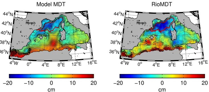
Fig. 1. Mean dynamic topography and geostrophic currents associated for the model (left) and Rio et al. (2007), (right). The bloom area is superimposed (red contour).
4o
W 0o
4oE 8oE 12oE 16oE 36o
N 38o
N 40o
N 42o
N 44o
N
Argo floats−2005
1st Jan 1st Mar 1st May
0 200 400 600 800
Depth (m)
4o
W 0o
4oE 8oE 12oE 16oE 36o
N 38o
N 40o
N 42o
N 44o
N
Argo floats−2008
1st Jan 1st Mar 1st May
0 200 400 600 800
Depth (m)
Fig. 2. Comparison between the mixed layer depth estimated from Argo floats data (circles) and that estimated by the model (asterisks) for the years 2005 and 2008. In the above panels the positions of the floats are displayed.
3 Data treatment
The present analysis is focused on the period from 1 De-cember to 31 May from 2001 to 2010 (9 yr), as we are in-terested in the interannual variability of spring bloom dy-namics. However, as the Aqua-MODIS data series starts in June 2002, this 9-yr period is reduced to 8 yr for the purpose of the satellite-model data comparison.
Hydrodynamic model results are validated by compari-son between modelled Mean Dynamic Topography (MDT)
[image:4.595.116.485.269.544.2]Table 1. Mean Mixed Layer Depth (MLD), mean daily vertically integrated nitrogen phytoplankton biomass (0–75 m, PHY) and primary production (0–75 m, PP), mean daily organic nitrogen export flux at 75 m depth (EF), mean daily neat heat flux (HF), mean daily wind speed (WS), day of the maximum MLD, week of the bloom onset for the model and for MODIS.
2002 2003 2004 2005 2006 2007 2008 2009 2010
MLD (m) 170 204 202 264 258 105 168 270 387
PHY (mmol N m−2) 43.5 41.9 44.2 42.5 41.7 46.3 45.4 41.1 39.3
PP (mmol N m−2day−1) 19.9 19.4 20.2 18.8 18.6 20.9 21.2 19.0 18.1
EF (mmol N m−2day−1) 4.63 3.88 5.77 5.79 7.38 6.23 9.07 8.02 7.26
HF (W m−2) −71 −80 −86 −109 −95 −42 −70 −100 −121
WS (m s−1) 6.11 6.10 6.29 6.46 6.35 5.69 6.38 7.15 7.56
Day max MLD 53 49 71 68 66 84 50 54 47
Week of bloom (model) 6 8 10 10 10 7 7 8 10
Week of bloom (MODIS) 8 10 10 11 8 6 3 8
To validate the model estimate of the Mixed Layer Depth (MLD) we use Argo floats data obtained from the Corio-lis Data Assembly Center. The float data are part of the MedArgo Programme (Poulain et al., 2007) started in 2003. We select float profiles for our specific bloom area and for the period of the simulation. The MLD is calculated (in both data and model) as the depth at which potential tempera-ture or potential density vary by more than1T =0.2◦C or 1σθ=0.03 kg m−3relative to their values at 10 m depth as
in de Boyer Montegut et al. (2004). The model output is sam-pled at the location and day of each valid Argo-float profile to allow model-data comparison (Fig. 2).
We use chlorophyll level-3 8-day composite maps from sensor Aqua-MODIS (2009.1 Ocean Colour Reprocessing) obtained from the NASA Ocean Colour Home Page. Im-ages are interpolated to the model grid because their reso-lution (∼1/16 pixel km−2) is higher than that of the model (∼1/23 pixel km−2). The data series obtained spans from June 2002 to December 2010 for a total of 391 maps. The sur-face chlorophyll estimated by the model is averaged at 8-day intervals to match the MODIS data series. Finally, MODIS data and model estimate are averaged over the area of the bloom and compared (Fig. 3).
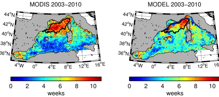
We calculate the maximum range of variability in the tim-ing of the bloom followtim-ing Henson et al. (2009). First, for each grid element, the onset of the bloom is determined for each year and for both series (model and MODIS). To this end, the method proposed by Siegel et al. (2002) is modified by considering the onset of the bloom as the first week of the year when the chlorophyll concentration is 10 % (instead of 5 %) above the median value for the period January–May (instead of the whole year). We obtain a map for each year (and both series) representing the onset date of the bloom. For each pixel the maximum and minimum values across the eight years are selected to define the maximum range of vari-ability in the bloom onset date over the period 2003–2010. These maps are shown in Fig. 4 with the area of the bloom superimposed for comparison.
2003 2004 2005 2006 2007 2008 2009 2010 0
0.3 0.6 0.9 1.2 1.5 1.8 2.1 2.4 2.7
Year
CHL (mg m
−
3)
Mean chl in bloom area
[image:5.595.311.544.250.387.2]MODIS Model
Fig. 3. MODIS and model chlorophyll concentration averaged over the area of the bloom. Only the period from 1 December to 31 May is shown for each year. As a consequence, the two series are not con-tinuous and the gray vertical bars represent the interruptions (from 31 May to 1 December).
In Table 1 we present a synthesis of model results that are used throughout the analysis. MLD is obtained from daily averages of temperature and salinity fields. The net heat flux (HF) represents the sum of shortwave and longwave radia-tion, latent and sensible heat assuming the positive sign for heat gained by the ocean. Wind speed (WS) is the magnitude of the resultant of the meridional and zonal components of the wind forcing applied to the model. MLD, HF and WS are presented as the average over the bloom area of daily mean values for each year. We present also the day of the max-imum MLD and the week of the bloom onset (referred to 1 January) for both the model and MODIS data. These dates are calculated also from the spatial average.
4o
W 0o
4oE 8oE 12oE 16oE
36o
N
38o
N
40o
N
42o
N
44o
N
MODIS 2003−2010
weeks
0 2 4 6 8 10
4o
W 0o
4oE 8oE 12oE 16oE
36o
N
38o
N
40o
N
42o
N
44o
N
MODEL 2003−2010
weeks
[image:6.595.115.473.61.220.2]0 2 4 6 8 10
Fig. 4. Maximum range of bloom start date from MODIS data (left) and model estimate (right).
and bacteria. It takes into account the vertical transport as a result of advection, diffusion and, for phytoplankton and detritus, gravitational sinking. Sinking can contribute only positively to the export flux while advection and diffusion can operate also upwards, giving rise to negative contribu-tions. In this sense, EF is a measure of the daily net vertical export flux of organic nitrogen at a fixed depth. We choose 75 m depth to characterise the export from the euphotic zone. The MLD during winter is almost always deeper than 75 m, thus, resuspension of organic nitrogen is very likely. How-ever, contributions to EF from resuspension are taken into account in the definition of EF itself. Another reason for the choice of the EF reference depth is that we are interested in mixing events that operate at daily timescale. Such mixing events are primarily wind-induced and their typical length-scale in the area during winter is ∼80 m according to the Obukhov length relation.
4 Results
The two MDT reproduce the main cyclonic circulation in the northern sector, roughly coinciding with the bloom area defined for this study (Fig. 1). In both model and data, the northern current originates in the NE sector after the join-ing of the eastern and western Corsican currents as described by Taupiere-Letage and Millot (1986). In the RioMDT the northern current is clearly visible along the northern coast from Italy up to the Ibiza channel while in the model MDT it appears somewhat more intense on the Italian coast and starts decreasing along the Spanish coast, in agreement with current measurements of∼5 cm s−1off the Ebro delta (Font et al., 1995). From climatological studies Font et al. (1988) described the deflection of one branch of the northern current that would then return cyclonically to the northeast to form the Balearic current. Both our model and data represent this deflection and the resultant Balearic current flowing towards the center of the Algero-Provenc¸al Basin. Here, between the
Balearic Islands and Corsica the mean flow is not well de-fined as this area is characterised by strong mesoscale circu-lation across the North Balearic frontal zone. The model de-picts a dominant NE flux that eventually joins the northward eastern Corsican current and closes the cyclonic circulation around the bloom area.
Model MLD is reasonably validated by ARGO float data. An example of this validation is shown in Fig. 2, for years 2005 and 2008. The model tends to overestimate the MLD throughout the winter in both years. Argo data and model estimates are significantly, though weakly, correlated in both cases (2005, r=0.33, p <0.05; 2008, r=0.23,
p <0.05). There is no clear difference in the mixed layer
evolution between the two years for both data and model. However, Argo-float data are sparse in space and the drift between subsequent profiles (up to 30 km) means they rarely profile the same water column twice (Smith et al., 2008). Furthermore, Argo floats drift with the prevailing currents and are found primarily in the southern and northern part of the bloom area during 2005 and 2008, respectively, along the path of the main cyclonic circulation. The northern sector is more directly exposed to the wind forcing than the southern side, suggesting that the representation of the mean mixed layer for the whole bloom area obtained from these loca-tions is likely to be negatively/positively biased respectively in 2005/2008.
−150 −100 −50 0 100
200 300 400
MLD (m)
HF (W m−2)
r=−0.96, p<0.01
−150 −100 −50 0
40 50 60 70 80
Bloom onset (day)
HF (W m−2)
r=−0.79, p<0.05
−150 −100 −50 0
18 19 20 21 22
PP (mmol N m
−
2 day
−
2 )
HF (W m−2)
r=0.88, p<0.01
−1502 −100 −50 0
4 6 8 10
EF (mmol N m
−
2 day
−
2 )
HF (W m−2)
[image:7.595.144.457.60.312.2]r=−0.17, p=0.65
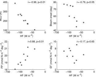
Fig. 5. Scatter plots of modelled heat fluxes vs. mixed layer depth (upper left), bloom onset date (upper right), primary production (lower left) and export flux (lower right). Each point represents the December through May average for an individual year (2002–2010). The bloom onset date is calculated as the first day that meets the chosen criteria for the bloom onset within the week identified as the first week of the bloom (see Sect. 3, “Data treatment”).
Gulf of Lions that roughly coincides with an area of well documented deep-water formation, often referred to as the MEDOC area (MEDOC, 1970). In this and other successive studies (Gascard, 1978; Marshall and Schott, 1999) the au-thors observed deep convection and a complete homogeniza-tion of the water column down to the bottom (>2000 m) over an area of 50–100 km in diameter. The model simulates deep homogenisation of the water column also in the Ligurian sub-basin, on the northeastern side of the bloom area. Recently, Smith et al. (2008) showed evidence of deep convection in the Western Ligurian subbasin during winter 2006 and in the Catalan Sea during winter 2005, both locations outside of the MEDOC area. Moreover, Hong et al. (2007) reported results from a numerical simulation showing how deep convection can extend into the Ligurian subbasin.
Surface chlorophyll estimated by the model and by MODIS averaged over the bloom area is shown in Fig. 3. The timing and intensity of the spring bloom is well captured by the model (r=0.76,p <0.01) although the yearly max-imum concentration is systematically underestimated. The interannual variability that determines the differences in the shape of the bloom seems to be reasonably captured by the model as the modest discontinuous blooms of 2003, 2007 and 2008 are clearly distinguishable from the shorter, more in-tense blooms of 2005, 2006 and 2010. In general, the model tends to overestimate surface chlorophyll during December, simulating a fall peak that is not observed in MODIS data.
The maximum range of variability in the timing of the bloom is shown for MODIS and model chlorophyll in Fig. 4. The bloom area is superimposed in both maps and shows, in the case of MODIS data, a strict coincidence with an area characterised by variability higher than 7–8 weeks. The model depicts a similar pattern, though more heterogeneous, with higher values (∼10 weeks) at the NE and SW sides and lower values (∼5–6 weeks) in the centre of the bloom area. When chlorophyll is averaged over the bloom area, the max-imum variability in the timing of the bloom is lower for both series as can be observed in Table 1. In this case, the agree-ment between MODIS and simulated data is generally good except for 2009 when a transient increase in MODIS chloro-phyll, on the third week, is wrongly interpreted as the onset of the bloom by our chosen criteria.
1st Jan 1st Feb 1st Mar 1st Apr 1st May 0
200
400
600
800
1000
1200
MLD (m)
year 2005
1st Jan 1st Feb 1st Mar 1st Apr 1st May
0 30 60 90 120
mmol N m
−
2
PHY EF PP MLD
1st Jan 1st Feb 1st Mar 1st Apr 1st May
0
200
400
600
800
1000
1200
MLD (m)
year 2008
1st Jan 1st Feb 1st Mar 1st Apr 1st May
0 30 60 90 120
mmol N m
−
2
[image:8.595.127.469.62.305.2]PHY EF PP MLD
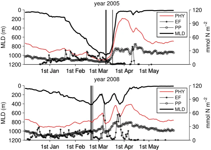
Fig. 6. Area averaged mixed layer depth (black continuous, left axis), vertically integrated phytoplankton nitrogen biomass (0–75 m, red continuous) and primary production (circles) and organic nitrogen export flux (asterisks) at 75 m depth. The period from December to May is shown for 2005 (above) and 2008 (below). The vertical bars represent the day of the bloom onset (thin) and the day of the maximum mixed layer depth.
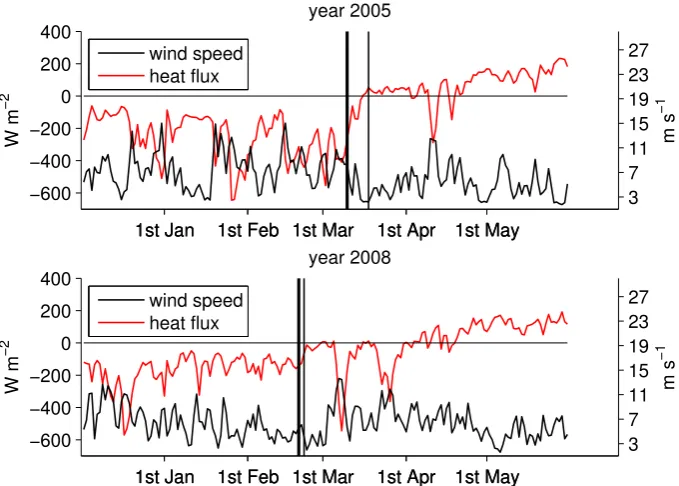
example of interannual variability. The relative differences between the two years in the mean MLD and heat flux are 57 % and 56 %, respectively. These two years also show very different bloom dynamics (Fig. 3).
The PP is fairly constant throughout the winter and tends to increase during the spring-bloom as can be observed for years 2005 and 2008 in Fig. 6. In both years (2005 and 2008) the peaks of EF are always associated to a sudden deepening of the mixed layer caused by a wind episode and the asso-ciated heat loss (Figs. 6 and 7). The vertical mixing redis-tributes the upper water column properties at depth resulting in a net downward transport of organic matter. This seems to affect the PP only partially, as PP never goes below a back-ground value close to the winter average. The model esti-mates a mean winter PP (December–February) ranging from 0.7 g C m−2d−1(2010) to 1.2 g C m−2d−1(2007) within the range of 0.1–2 g C m−2d−1measured by Mor´an and Estrada (2005) in winter for the NW Mediterranean.
The simulated export flux are comparable to sediment trap data collected in the bloom area. Lee et al. (2009) reported a mean daily export of organic carbon of∼29 mg C m−2d−1 for the period March–May 2003 at 238 m depth at the DY-FAMED station in the northeastern sector of the bloom area. The model estimates a mean EF of particulate organic car-bon of∼40 mg C m−2d−1 at the same depth, location and for the same period. Data from a neighbouring area, but from sediment traps deployed just below the euphotic zone (80 m) were presented by Miquel et al. (1994) for the
pe-riod between mid April 1987 and mid November 1988. The authors reported for the second half of April 1987 a mean export of ∼4 mg N m−2d−1. The model estimate for the same period averaged over the 10 yr of the simulation gives ∼6.4 mg N m−2d−1.
In Fig. 8 we show the cumulative export flux for years 2001 to 2010, the 10 yr mean, and the maximum range of interannual variability calculated as the difference be-tween the year with the highest value and the year with the lowest value (at each day). The cumulative EF grows throughout the winter and stabilises in April as vertical mix-ing decreases. The final maximum range of interannual vari-ability is around 800 mmol N m−2(∼66 % of the final mean accumulated EF), half of which is accumulated during De-cember and the other half during March. Although the cu-mulative EF keeps growing during January and February, the maximum range of interannual variability is almost constant during this period (dotted line, Fig. 8). We focus the dis-cussion on the export flux, excluding the contribution from December because this is likely to be affected by the model overestimation of phytoplankton biomass during this period.
5 Discussion
1st Jan 1st Feb 1st Mar 1st Apr 1st May −600
−400 −200 0 200 400
W m
−
2
year 2005
1st Jan 1st Feb 1st Mar 1st Apr 1st May
3 7 11 15 19 23 27
m s
−
1
wind speed heat flux
1st Jan 1st Feb 1st Mar 1st Apr 1st May
−600 −400 −200 0 200 400
W m
−
2
year 2008
1st Jan 1st Feb 1st Mar 1st Apr 1st May
3 7 11 15 19 23 27
m s
−
1
[image:9.595.129.469.62.305.2]wind speed heat flux
Fig. 7. Model daily neat heat flux and mean wind speed averaged over the area of the bloom for the years 2005 (above) and 2008 (below). The vertical lines represent the day of the maximum MLD (thick line) and the spring bloom onset date (thin line).
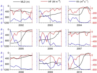
et al. (2006) in the sense that a deeper mixed layer would take longer to re-stratify and thus would result in a later bloom. However, pulses of high primary production have often been observed in absence of thermal stratification (Townsend et al., 1992; Eilertsen, 1993; Dale et al., 1999; Koertzinger et al., 2008) demonstrating that a shallow mixed layer is not a necessary condition for a bloom to start. Huis-man et al. (1999) and more recently Taylor and Ferrari (2011) related the beginning of the bloom to a critical threshold of turbulent diffusivity coinciding with the decrease of the heat loss to the atmosphere. Crucial to their analysis is the dis-tinction between a mixed layer with a uniform density and a mixing layer with a uniform density and active turbulence (Brainerd and Gregg, 1995). In other words, there is a time-lag between the shutting off of the heat loss from the sea sur-face and the re-stratification. During this time the low active turbulence allows an increase in the average time of expo-sure of phytoplankton to light even if the mixed layer is still deep. Our results confirm that a condition of close-to-zero heat flux is indeed a better estimator than the mixed layer depth for the onset of the bloom (Fig. 9). Also the onset of the bloom is clearly associated with a significant drop in the vertical diffusivity which depends on the turbulent kinetic en-ergy, as posited by Taylor and Ferrari (2011). Although we do not explicitly calculate the Sverdrup’s critical depth, Fig. 9 shows how the bloom can start even when the mixed layer is still several hundred metres deep as long as the heat flux ap-proaches zero and the vertical diffusivity is low. Since the timing of the bloom is independent of the depth of the mixed
1st Jan 1st Feb 1st Mar 1st Apr 1st May 0
400 800 1200 1600
mmol N m
−
2
Fig. 8. Cumulative EF for each year (thin lines), their average (dots) and the maximum range of variability (thick line – i.e., the high-est year minus the lowhigh-est at each day). Circles represent the spring bloom onset date for each year.
layer, we conclude that there is no preconditioning effect on the timing of the bloom.
[image:9.595.310.545.364.484.2]0 0.4 0.8 1.2 1.6
2002 0
400
800
1200
MLD (m)
2003 HF (W m−2)
−600 −400 −200 0
2004 Kh (m2 s−1)
0 0.4 0.8 1.2 1.6
2005 0
400
800
1200
2006
−600 −400 −200 0
2007
0 0.4 0.8 1.2 1.6
2008 0
400
800
1200
2009
−600 −400 −200 0
[image:10.595.131.468.64.316.2]2010
Fig. 9. Detail of heat flux (HF, red), mixed layer depth (MLD, black) and vertical diffusivity (mean 0–75 m depth, Kh, blue) from 10 days before up to 10 days after the onset of the bloom (vertical black thin line). The zero heat flux line is also shown for reference (horizontal black thin line).
10 20 30 40 50 60 70
3 6 9 12 15 18 21
EF (mmol N m
−
2 day
−
1)
Frequency of windy days (%)
Fig. 10. Mean daily March EF (on the abscissa) and frequency of days during March with wind above the daily March 10-yr average (on the ordinate).
decrease in wind together with an increase in solar radiation result in a sign inversion in the heat flux and a marked drop in the turbulent diffusivity. The same mechanism occurs in 2008 but 3 weeks earlier.
In our example, winter 2005 is colder than winter 2008 and a higher portion of the winter is characterised by intense wind forcing, higher heat loss and hence a deeper mixed layer.
In winter 2008 a less intense storminess both decreases the mean MLD and increases the probability of an early onset of the bloom. We suggest then that a deeper mixed layer and a later bloom are both consequences of a long and intense winter forcing, but are not directly related as the maximum MLD has no direct influence on the timing of the bloom.
[image:10.595.49.286.381.569.2]Our model results indicate that export flux is driven by a combination of available surface biomass and vertical mix-ing. During January and February, EF stays at a background level, very close to PP indicating that mixed conditions are favourable to an efficient transport of organic matter at depth. No interannual variability is added during these two months because those years characterised by more intense winter mixing (i.e., 2005) tend to have lower surface biomass than those years characterised by a shallower winter mixed layer (i.e., 2008). Since EF is driven by a combination between biomass availability at the surface and vertical mixing, the result is a compensation that leads to an almost year-to-year constant winter EF. This compensation partly explains why EF is not correlated with HF in Fig. 5.
About half of the maximum range of interannual variabil-ity in EF is accumulated in March (Fig. 8). In particular, in-terruptions of the bloom as observed in March 2008 are asso-ciated to the peaks in EF that are responsible for this half of the interannual variability. We have found that the portion of interannual variability in EF, accumulated in March, is deter-mined by the interannual variability in wind forcing during this month. The frequency of windy days during March, cal-culated as the percentage of days with average wind above the 10-yr average mean daily value for the same month, cor-relates well (r=0.9, p <0.01) with the March mean daily EF (Fig. 10).
Therefore, March is a key period during which a signifi-cant part of the interannual variability in the total EF is de-termined. This is because the range of variability in the date of the bloom onset is centred on the first week of this month (week 8.4, average blooming week in Table 1) amplifying the effect of the interannual variability of wind-induced mixing episodes on EF. In other words, the bloom has already started during, at least, a part of March, every year. This means that there is abundance of surface biomass to be exported at depth by eventual wind-driven mixing episodes.
Importantly, our results suggest that satellite chlorophyll could be used to identify years with higher EF. Counter-intuitively, years with a bloom of intermittent nature char-acterised by low maximum chlorophyll concentrations are likely to also be years of high EF while years characterised by an intense uninterrupted bloom would have lower EF.
The bloom area considered in this study lies between 40.5◦N and 44◦N. Henson et al. (2009) defined a tran-sition zone in the North Atlantic between 40◦N and 45◦N, based on the significance of the temporal correla-tion between weekly SeaWiFS chlorophyll concentracorrela-tion and MLD estimated from optimally interpolated Argo float data. North/south of this transition zone the correlation was negative/positive as expected for a subpolar (light lim-ited)/subtropical (nutrient limited) environment. The same correlation for our model results (not shown) shows a vari-able (∼0–0.5), primarily negative correlation in the bloom area. This suggests that this area encompasses a variety of behaviours ranging from the southern subpolar up to the
tran-sitional. We, therefore, emphasise the relevance of our results also for an important portion of the North Atlantic where high interannual variability has been observed in the tim-ing and intensity of the sprtim-ing bloom (Henson et al., 2009; Ueyama and Monger, 2005).
Shifts in storm tracks and modes of atmospheric circu-lation are responsible for the interannual variability in the passage of weather systems. The transition to springtime is a critical moment when the passage of these weather sys-tems is able to modulate bloom dynamics and consequently the vertical export of organic matter.
6 Conclusions
Model results show a clear connection between the year-to-year variability of the spring phytoplankton bloom and the year-to-year variability of the vertical export flux of organic matter. Late blooms and deep mixed layers are both the re-sult of intense wind forcing, but are not necessarily related to each other. A condition of close-to-zero surface heat flux as postulated by Taylor and Ferrari (2011) seems to be a better predictor for the bloom timing than the onset of stratification. The bloom onset is centred, on average, on the first week of March with earlier blooms starting during low-wind periods in February. The frequency of wind episodes is a key factor controlling the onset and the following development of the bloom. The passage of weather systems in the transition from winter to spring can interrupt the development of the bloom by actively mixing phytoplankton at depth. This results in a net vertical export of organic matter, driven by a combi-nation of surface biomass availability and vertical mixing. Since the bloom has already started during at least some part of March each year, the frequency of wind-driven mixing episodes during this month has a strong impact on the export flux accumulated in winter-spring. Our simulation shows that at least half of the maximum interannual variability in this flux is determined during March. Importantly and perhaps counterintuitively, our results show that years with less in-tense and discontinuous blooms are likely to have higher ex-port flux than years with intense uninterrupted blooms.
Acknowledgements. The simulations were performed on the supercomputer FinisTerrae hosted at the Centre of Supercomputing of Galicia (CESGA) and financed by the regional government of Galicia and the Spanish National Research Council (CSIC). This work was partly funded by the Spanish Ministry of Science and Innovation project “Observation, analysis and modelling of the Mediterranean Sea – OAMMS” CTM2008–03983. The first author (R.B.) would like to thank the Catalan regional government for financial support through the program FI. The authors would also like to thank two anonymous reviewers who helped to improve the manuscript.
References
Amante, C. and Eakins, B. W.: ETOPO1 1 Arc-Minute Global Re-lief Model: Procedures, Data Sources and Analysis, NGDC 24, NOAA, 2009.
Anderson, T. R.: Modelling the influence of food C:N ratio, and respiration on growth and nitrogen excretion in marine zooplankton and bacteria, J. Plankton Res., 14, 1645–1671, doi:10.1093/plankt/14.12.1645, 1992.
Baham´on, N. and Cruzado, A.: Modelling nitrogen fluxes in oligotrophic environments: NW Mediterranean and NE Atlantic, Ecol. Model., 163, 223–244, doi:10.1016/S0304-3800(03)00007-3, 2003.
Barale, V., Jaquet, J.-M., and Ndiaye, M.: Algal blooming patterns and anomalies in the Mediterranean Sea as derived from the Sea-WiFS data set (1998–2003), Remote Sens. Environ., 112, 3300– 3313, doi:10.1016/j.rse.2007.10.014, 2008.
Bernardello, R.: A 3D high resolution coupled hydrodynamicbio-geochemical model for the Western Mediterranean Sea. Interan-nual variability of primary and export production., Ph.D. thesis, Universitat Politecnica de Catalunya, Barcelona, Spain, 2010. Bishop, J., Conte, M. H., Wiebe, P., Roman, M., and Langdon, C.:
Particulate matter production and consumption in deep mixed layers – observations in a warm-core ring, Deep-Sea Res., 33, 1813–1841, doi:10.1016/0198-0149(86)90081-6, 1986. Blumberg, A. F. and Mellor, G. L.: A description of a
three-dimensional coastal ocean circulation model, in: Three-dimensional Coastal Ocean Models, edited by: Heaps, N. S., American Geophysical Union, 1–16, 1987.
Bosc, E., Bricaud, A., and Antoine, D.: Seasonal and inter-annual variability in algal biomass and primary production in the Mediterranean Sea, as derived from 4 years of Sea-WiFS observations, Global Biogeochem. Cy., 18, GB1005, doi:10.1029/2003GB002034, 2004.
Brainerd, K. and Gregg, M.: Surface mixed and mixing layer depths, Deep-Sea Res. Pt. I, 42, 1521–1543, doi:10.1016/0967-0637(95)00068-H, 1995.
Dale, T., Rey, F., and Heimdal, B.: Seasonal development of phy-toplankton at a high latitude oceanic site, Sarsia, 84, 419–435, 1999.
de Boyer Montegut, C., Madec, G., Fischer, A. S., Lazar, A., and Iu-dicone, D.: Mixed layer depth over the global ocean: an examina-tion of profile data and a profile-based climatology, J. Geophys. Res., 109, C12003, doi:10.1029/2004JC002378, 2004.
D’Ortenzio, F. and Ribera d’Alcal`a, M.: On the trophic regimes of the Mediterranean Sea: a satellite analysis, Biogeosciences, 6, 139–148, doi:10.5194/bg-6-139-2009, 2009.
D’Ortenzio, F., Iudicone, D., de Boyer-Montegut, C., Testor, P., An-toine, D., Marullo, S., Santoleri, R., and Madec, G.: Seasonal variability of the mixed layer depth in the Mediterranean Sea as derived from in situ profiles, Geophys. Res. Lett., 32, L12605, doi:10.1029/2005GL022463, 2005.
Dutkiewicz, S., Follows, M., Marshall, J., and Gregg, W. W.: Inter-annual variability of phytoplankton abundances in the North At-lantic, Deep-Sea Res. Pt. II, 48, 2323–2344, doi:10.1016/S0967-0645(00)00178-8, 2001.
Eilertsen, H.: Spring blooms and stratification, Nature, 363, 24, 1993.
Estournel, C., Auclair, F., Lux, M., Nguyen, C., and Marsaleix, P.: “Scale oriented” embedded modeling of the North-Western
Mediterranean in the frame of MFSTEP, Ocean Sci., 5, 73–90, doi:10.5194/os-5-73-2009, 2009.
Fasham, M. J. R., Ducklow, H. W., and McKelvie, S. M.: A nitrogen-based model of plankton dynamics in the ocean mixed layer, J. Mar. Res., 48, 591–639, 1990.
Font, J., Salat, J., and Tintor´e, J.: Permanent features of the circula-tion in the Catalan Sea, Oceanol. Acta, 9, 51–57, 1988. Font, J., Garcia-Ladona, E., and Gorriz, E.: The seasonality of
mesoscale motion in the Northern Current of the Western Mediterranean: several years of evidence, Oceanol. Acta, 18, 207–219, 1995.
Gardner, W. D., Chung, S. P., Richardson, M. J., and Walsh, I. D.: The oceanic mixed-layer pump, Deep-Sea Res. Pt. II, 42, 757– 775, doi:10.1016/0967-0645(95)00037-Q, 1995.
Gascard, J.: Mediterranean deep-water formation baroclinic insta-bility and oceanic eddies, Oceanol. Acta, 1, 315–330, 1978. Henson, S. A., Robinson, I., Allen, J. T., and Waniek, J. J.:
Ef-fect of meteorological conditions on interannual variability in timing and magnitude of the spring bloom in the Irminger Basin, North Atlantic, Deep-Sea Res. Pt. I, 53, 1601–1615, doi:10.1016/j.dsr.2006.07.009, 2006.
Henson, S. A., Dunne, J. P., and Sarmiento, J. L.: Decadal variabil-ity in North Atlantic phytoplankton blooms, J. Geophys. Res.-Oceans, 114, C04013, doi:10.1029/2008JC005139, 2009. Ho, C. and Marra, J.: Early-spring export of phytoplankton
produc-tion in the Northeast Atlantic-ocean, Mar. Ecol.-Prog. Ser., 114, 197–202, doi:10.3354/meps114197, 1994.
Hong, X., Hodur, R. M., and Martin, P. J.: Numerical simulation of deep-water convection in the Gulf of Lion, Pure Appl. Geophys., 164, 2101–2116, doi:10.1007/s00024-007-0261-0, 2007. Huisman, J., van Oostveen, P., and Weissing, F.: Critical depth and
critical turbulence: two different mechanisms for the develop-ment of phytoplankton blooms, Limnol. Oceanogr., 44, 1781– 1787, 1999.
Jordi, A. and Wang, D. P.: sbPOM: A parallel implementation of Princenton Ocean Model, Environ. Modell. Softw., 38, 59–61, doi:10.1016/j.envsoft.2012.05.013, 2012.
Koertzinger, A., Send, U., Lampitt, R. S., Hartman, S., Wal-lace, D. W. R., Karstensen, J., Villagarcia, M. G., Llinas, O., and DeGrandpre, M. D.: The seasonal pCO(2) cycle at 49 de-grees N/16.5 dede-grees W in the Northeastern Atlantic Ocean and what it tells us about biological productivity, J. Geophys. Res.-Oceans, 113, C04020, doi:10.1029/2007JC004347, 2008. Koeve, W., Pollehne, F., Oschlies, A., and Zeitzschel, B.:
Storm-induced convective export of organic matter during spring in the Northeast Atlantic Ocean, Deep-Sea Res. Pt. I, 49, 1431–1444, doi:10.1016/S0967-0637(02)00022-5, 2002.
Leaman, K. D. and Schott, F. A.: Hydrographic structure of the convection regime in the Gulf of Lions: winter 1987, J. Phys. Oceanogr., 21, 575–598, doi:10.1175/1520-0485(1991)021<0575:HSOTCR>2.0.CO;2, 1991.
Lee, C., Armstrong, R. A., Cochran, J. K., Engel, A., Fowler, S. W., Goutx, M., Masqu´e, P., Miquel, J. C., Peterson, M., Tam-burini, C., and Wakeham, S.: MedFlux: investigations of particle flux in the Twilight Zone, Deep-Sea Res. Pt. II, 56, 1363–1368, doi:10.1016/j.dsr2.2008.12.003, 2009.
the climatology of water masses and to validate incoming data from operational oceanography, J. Marine Syst., 48, 83–116, doi:10.1016/j.jmarsys.2003.11.025, 2004.
Marshall, J. and Schott, F.: Open-ocean convection: obser-vations, theory, and models, Rev. Geophys., 37, 1–64, doi:10.1029/98RG02739, 1999.
MEDOC: Observation of formation of deep water in the Mediter-ranean Sea, 1969, Nature, 227, 1037–1040, 1970.
Mertens, C. and Schott, F.: Interannual variability of deep-water formation in the Northwestern Mediterranean, J. Phys. Oceanogr., 28, 1410–1424, doi:10.1175/1520-0485(1998)028<1410:IVODWF>2.0.CO;2, 1998.
Millot, C.: Circulation in the Western Mediterranean Sea, J. Marine Syst., 20, 423–442, doi:10.1016/S0924-7963(98)00078-5, 1999. Miquel, J., Fowler, S., Rosa, J. L., and Buat-Menard, P.: Dynamics of the downward flux of particles and carbon in the open North-western Mediterranean Sea, Deep-Sea Res. Pt. I, 41, 243–261, doi:10.1016/0967-0637(94)90002-7, 1994.
Mor´an, X. A. G. and Estrada, M.: Winter pelagic photosynthesis in the NW Mediterranean, Deep-Sea Res. Pt. I, 52, 1806–1822, doi:10.1016/j.dsr.2005.05.009, 2005.
Pinardi, N. and Coppini, G.: Preface “Operational oceanography in the Mediterranean Sea: the second stage of development”, Ocean Sci., 6, 263–267, doi:10.5194/os-6-263-2010, 2010.
Poulain, P.-M., Barbanti, R., Font, J., Cruzado, A., Millot, C., Gert-man, I., Griffa, A., Molcard, A., Rupolo, V., Le Bras, S., and Petit de la Villeon, L.: MedArgo: a drifting profiler program in the Mediterranean Sea, Ocean Sci., 3, 379–395, doi:10.5194/os-3-379-2007, 2007.
Rio, M.-H., Poulain, P.-M., Pascual, A., Mauri, E., Larnicol, G., and Santoleri, R.: A mean dynamic topography of the Mediter-ranean Sea computed from altimetric data, in-situ measurements and a general circulation model, J. Marine Syst., 65, 484–508, doi:10.1016/j.jmarsys.2005.02.006, 2007.
Siegel, D. A., Doney, S. C., and Yoder, J. A.: The North Atlantic spring phytoplankton bloom and Sverdrup’s Critical Depth Hy-pothesis, Science, 296, 730–733, 2002.
Simonot, J., Dollinger, E. and Le Treut, H.: Thermodynamic-Biological-Optical Coupling in the Oceanic Mixed Layer, J. Geo-phys. Res., 93, 8193–8202, 1988.
Smith, R. O., Bryden, H. L., and Stansfield, K.: Observations of new western Mediterranean deep water formation using Argo floats 2004–2006, Ocean Sci., 4, 133–149, doi:10.5194/os-4-133-2008, 2008.
Sverdrup, H. U.: On conditions for the vernal blooming of phyto-plankton, J. Conseil, 18, 287–295, 1953.
Takahashi, T., Sutherland, S. C., Wanninkhof, R., Sweeney, C., Feely, R. A., Chipman, D. W., Hales, B., Friederich, G., Chavez, F., Sabine, C., Watson, A., Bakker, D. C. E., Schuster, U., Metzl, N., Yoshikawa-Inoue, H., Ishii, M., Midorikawa, T., Nojiri, Y., Koertzinger, A., Steinhoff, T., Hoppema, M., Olafsson, J., Arnarson, T. S., Tilbrook B., Jo-hannessen, T., Olsen, A., Bellerby, R., Wong, C. S., Delille, B., Bates, N. R., and de Baar, H. J. W.: Climatological mean and decadal change in surface ocean pCO(2), and net sea-air CO2 flux over the global oceans, Deep-Sea Res. Pt. II, 56, 554–577, doi:10.1016/j.dsr2.2008.12.009, 2009.
Taupiere-Letage, I. and Millot, C.: General hydrodynamical fea-tures in the Ligurian Sea inferred from the DYOME experiment, Oceanol. Acta, 9, 119–131, 1986.
Taylor, J. R. and Ferrari, R.: Shutdown of turbulent con-vection as a new criterion for the onset of spring phy-toplankton blooms, Limnol. Oceanogr., 56, 2293–2307, doi:10.4319/lo.2011.56.6.2293, 2011.
Tonani, M., Pinardi, N., Dobricic, S., Pujol, I., and Fratianni, C.: A high-resolution free-surface model of the Mediterranean Sea, Ocean Sci., 4, 1–14, doi:10.5194/os-4-1-2008, 2008.
Tonani, M., Pinardi, N., Fratianni, C., Pistoia, J., Dobricic, S., Pensieri, S., de Alfonso, M., and Nittis, K.: Mediterranean Forecasting System: forecast and analysis assessment through skill scores, Ocean Sci., 5, 649–660, doi:10.5194/os-5-649-2009, 2009.
Townsend, D. W., Keller, M. D., Sieracki, M. E., and Ack-leson, S. G.: Spring phytoplankton blooms in the absence of vertical water column stratification, Nature, 360, 59–62, doi:10.1038/360059a0, 1992.
Ueyama, R. and Monger, B. C.: Wind-induced modulation of sea-sonal phytoplankton blooms in the North Atlantic derived from satellite observations, Limnol. Oceanogr., 50, 1820–1829, 2005. Varela, R. A., Cruzado, A., Tintor´e, J., and Garc´ıa Ladona, E.: Modelling the deep-chlorophyll maximum: a coupled physical-biological approach, J. Mar. Res., 50, 441–463, 1992.
Volpe, G., Nardelli, B. B., Cipollini, P., Santoleri, R., and Robinson, I. S.: Seasonal to interannual phytoplankton re-sponse to physical processes in the Mediterranean Sea from satellite observations, Remote Sens. Environ., 117, 223–235, doi:10.1016/j.rse.2011.09.020, 2012.