Module – 3 Lecture Notes – 2
Graphical Method
Graphical method to solve Linear Programming problem (LPP) helps to visualize the
procedure explicitly. It also helps to understand the different terminologies associated with the solution of LPP. In this class, these aspects will be discussed with the help of an example. However, this visualization is possible for a maximum of two decision variables. Thus, a LPP with two decision variables is opted for discussion. However, the basic principle remains the same for more than two decision variables also, even though the visualization beyond two-dimensional case is not easily possible.
Let us consider the same LPP (general form) discussed in previous class, stated here once again for convenience.
5) (C & 4) (C 0 , 3) (C 15 4 2) (C 11 3 1) (C 5 3 2 to subject 5 6 Maximize − − ≥ − ≤ + − ≤ + − ≤ − + = y x y x y x y x y x Z
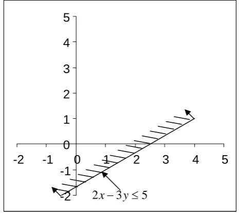
First step to solve above LPP by graphical method, is to plot the inequality constraints one-by-one on a graph paper. Fig. 1a shows one such plotted constraint.
5 3 2x− y≤ -2 -1 0 1 2 3 4 5
-2 -1 0 1 2 3 4 5
Fig. 1a Plot showing first constraint (2x−3y≤5)
Fig. 1b shows all the constraints including the nonnegativity of the decision variables (i.e.,
and ).
0
≥
x+3y≤11
4x+ y≤15
x≥0
y≥0
2x−3y≤5 -2
-1 0 1 2 3 4 5
-2 -1 0 1 2 3 4 5
Fig. 1b Plot of all the constraints
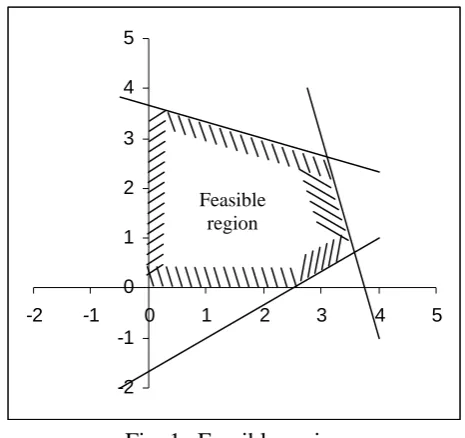
Common region of all these constraints is known as feasible region (Fig. 1c). Feasible region implies that each and every point in this region satisfies all the constraints involved in the LPP.
-2 -1 0 1 2 3 4 5
-2 -1 0 1 2 3 4 5
Feasible region
Fig. 1c Feasible region
y axis is 3. If,
5 5 6
5 5
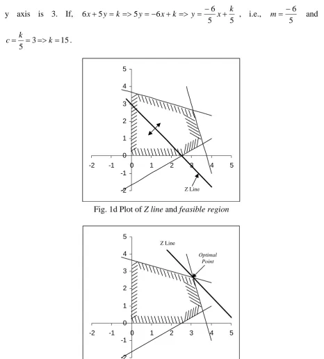
6x+ y=k => y =− x+k => y= −6x+k , i.e.,
5
=
m −6 and
15 3
5 = => =
= k
c k .
-2 3 4 5
-2 0 1 2 3 4 5
-1 0 1 2
-1
Z Line
Fig. 1d Plot of Z line and feasible region
-2 -1 0 1 2 3 4 5
-2 -1 0 1 2 3 4 5
Optimal Point
Z Line
Fig. 1e Location of Optimal Point
Now it can be visually noticed that value of the objective function will be maximum when it passes through the intersection of x+3y=11 and 4x+ =y 15
*
x y* =2.636
* *
5 6x + y
=
(straight lines associated with the second and third inequality constraints). This is known as optimal point (Fig. 1e). Thus the optimal point of the present problem is and . And the optimal solution is = 31.727
091 . 3
Visual representation of different cases of solution of LPP
A linear programming problem may have i) a unique, finite solution, ii) an unbounded solution iii) multiple (or infinite) number of optimal solutions, iv) infeasible solution and v) a unique feasible point. In the context of graphical method it is easy to visually demonstrate the different situations which may result in different types of solutions.
Unique, finite solution
The example demonstrated above is an example of LPP having a unique, finite solution. In such cases, optimum value occurs at an extreme point or vertex of the feasible region.
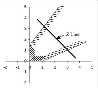
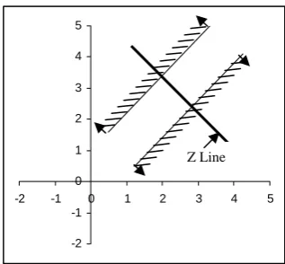
Unbounded solution
If the feasible region is not bounded, it is possible that the value of the objective function goes on increasing without leaving the feasible region. This is known as unbounded solution (Fig 2).
-2 -1 0 1 2 3 4 5
-2 -1 0 1 2 3 4 5
Z Line
Multiple (infinite) solutions
If the Z line is parallel to any side of the feasible region all the points lying on that side constitute optimal solutions as shown in Fig 3.
-2 -1 0 1 2 3 4 5
-2 -1 0 1 2 3 4 5
Parallel
Z Line
Fig. 3 Multiple (infinite) Solution Infeasible solution
Sometimes, the set of constraints does not form a feasible region at all due to inconsistency in the constraints. In such situation the LPP is said to have infeasible solution. Fig 4 illustrates such a situation.
-2 -1 0 1 2 3 4 5
-2 -1 0 1 2 3 4 5
Z Line
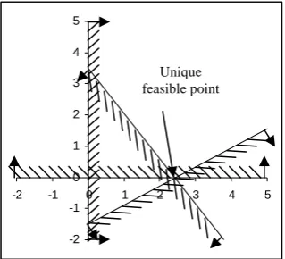
Unique feasible point
This situation arises when feasible region consist of a single point. This situation may occur only when number of constraints is at least equal to the number of decision variables. An example is shown in Fig 5. In this case, there is no need for optimization as there is only one solution.
-2 -1 0 1 2 3 4 5
-2 -1 0 1 2 3 4 5
Unique feasible point