https://doi.org/10.3926/jiem.2944
Key Issues on Partial Least Squares (PLS) in Operations Management
Research: A Guide to Submissions
Juan A. Marin-Garcia1 , Rafaela Alfalla-Luque2
1ROGLE. Dpto. de Organización de Empresas. Universitat Politècnica de València (Spain)
2GIDEAO Research Group, Departamento de Economía Financiera y Dirección de Operaciones Universidad de Sevilla (Spain)
[email protected], [email protected]
Received: February 2019 Accepted: May 2019
Abstract:
Purpose: This work aims to systematise the use of PLS as an analysis tool via a usage guide or recommendation for researchers to help them eliminate errors when using this tool.
Design/methodology/approach: A recent literature review about PLS and discussion with experts in the methodology.
Findings:This article considers the current situation of PLS after intense academic debate in recent years, and summarises recommendations to properly conduct and report a research work that uses this methodology in its analyses. We particularly focus on how to: choose the construct type; choose the estimation technique (PLS or CB-SEM); evaluate and report the measurement model; evaluate and report the structural model; analyse statistical power.
Research limitations: It was impossible to cover some relevant aspects in considerable detail herein: presenting a guided example that respects all the report recommendations presented herein to act as a practical guide for authors; does the specification or evaluation of the measurement model differ when it deals with first-order or second-order constructs?; how are the outcomes of the constructs interpreted with the indicators being measured with nominal measurement levels?; is the Confirmatory Composite Analysis approach compatible with recent proposals about the Confirmatory Tetrad Analysis (CTA)? These themes will the object of later publications.
Originality/value: We provide a check list of the information elements that must contain any article using PLS. Our intention is for the article to act as a guide for the researchers and possible authors who send works to the JIEM (Journal of Industrial and Engineering Management). This guide could be used by both editors and reviewers of JIEM, or other journals in this area, to evaluate and reduce the risk of bias (Losilla, Oliveras, Marin-Garcia & Vives, 2018) in works using PLS as an analysis procedure.
Keywords:PLS-SEM, Partial Least Squares, operations management, reporting standards
To cite this article:
Marin-Garcia, J.A., & Alfalla-Luque, R. (2019). Key issues on Partial Least Squares (PLS) in operations management research: A guide to submissions. Journal of Industrial Engineering and Management, 12(2), 219-240.
1. Introduction
This leading article is based on an article previously published by the authors in the journal WPOM (Marín-García & Alfalla-Luque, 2019). The original article was published in Spanish with further information to that mentioned herein. We republished this work with adaptations for JIEM and translated it into English for more widely disseminate it to a different group of researchers whose access to the original article would not be easy (Callahan, 2018), (similar examples are (González De Dios, 2011; Moher, Liberati, Tetzlaff, Altman & The, 2009; Urrútia & Bonfill, 2010, 2013), or (Welch, Petticrew, Petkovic, Moher, Waters, White et al., 2015, 2016a., 2016b; Welch, Petticrew, Tugwell, Moher, O’Neill, Waters et al., 2012, 2013), or (Moher, Shamseer, Clarke, Ghersi, Liberati, Petticrew et al., 2015, 2016). As some sections in both articles overlap and complement one another, we recommend citing both articles to refer to their contributions.
Extending structural equations models based on composites (PLS-SEM) has been widely diffused of late in areas like marketing (Hair, Sarstedt, Ringle & Mena, 2012b; Henseler, Ringle & Sinkovics, 2009; Hult, Hair, Proksch, Sarstedt, Pinkwart & Ringle, 2018), information systems (Petter, 2018; Ringle, Sarstedt & Straub, 2012; Roldán & Sánchez-Franco, 2012; Sharma, Sarstedt, Shmueli, Kim & Thiele, 2019; Urbach & Ahleman, 2010), tourism (do Valle & Assaker, 2016; Duarte & Amaro, 2018; Kumar & Purani, 2018; Latan, 2018; Usakli & Kucukergin, 2018), health sciences (Avkiran, 2018) or human resources (Ringle, Sarstedt, Mitchell, & Gudergan, 2018), among others. The two most recent reviews in the operations management area (Kaufmann & Gaeckler, 2015; Peng & Lai, 2012) came prior to intense debate about the methodology that shook the Partial Least Squares (PLS) community between 2014 and 2018. New tools continue to be developed and modifications to the report standards of articles made using PLS as an analysis tool are established.
This work aims to systematise the use of PLS as an analysis tool via a usage guide or recommendation for researchers to help them eliminate errors when using this tool. This guide could be used by editors and reviewers of JIEM, or other journals in the area, to evaluate and reduce the risk of bias (Losilla et al., 2018) of works using PLS as an analysis procedure.
2. PLS as an Analysis Tool
The PLS method consists in a sequence of multiple regressions that allows the weights of construct components (when reaching the predefined level of convergence) and paths to be estimated between exogenous and endogenous constructs (Esposito-Vinzi, Chin, Henseler & Wang, 2010; Felipe, Roldán & Leal-Rodríguez, 2017; Henseler et al., 2009). The algorithm is developed in several stages. The first stage iteratively estimates the Latent Variable Scores (LVS). The second stage solves the measurement model by estimating outer weights and loadings (beginning with the LVS estimated in the first stage). The third stage estimates the parameters of the structural model (Hair, Hult, Ringle & Sarstedt, 2017; Ringle, Wende & Becker, 2015).
PLS is one of the methods in the variance-based structural equations family (SEM). One of its most outstanding aspects is that it is a method based on composites instead of common (reflective) factors or causal formative constructs. However, this does not represent a limitation when attempting to test models whose constructs match a composites typology (Henseler, 2017a; Rigdon, 2012, 2014; Sarstedt, Hair, Ringle, Thiele & Gudergan, 2016). Along these lines, PLS allows weights based on correlations (Mode A) or regressions (Mode B) to be estimated, or to correct with PLSc (consistent PLS) the correlations of those constructs specified as common factors to make the results consistent with that measurement model (Dijkstra & Henseler, 2015a; Dijkstra & Henseler, 2015b). This provides versatility when analysing mixed models where the constructs that are present are composites (when indicators are poorly correlated and if indicators present a moderate-high correlation of the sample being worked with) and also common factors (Rigdon, Sarstedt & Ringle, 2017).
predictor constructs), although alternatives based on Two-Stage Least Squares has become popular (Henseler & Roldan, 2017). We hope that debate will commence in the future about these and other alternatives to mathematically solve a usual conceptual problem in operations management, where we cannot always contemplate how exogenous constructs are orthogonal (no correlation among them).
Another characteristic of a composite-based analysis is that it allows LVS to be calculated as an exact linear combination of the observed variables so that they are never indeterminate and can be used in subsequent analyses (either in aggregation stages in second-or third-order constructs or with other statistical procedures that differ from structural equations) (Chin, 1998; Hair, Risher, Sarstedt & Ringle, 2019b; Richter, Cepeda, Roldán & Ringle, 2016).
One useful aspect to stress is that PLS allows exogenous (predictor) constructs to be used whose indicators are measured at any measurement level (nominal, ordinal, interval or ratio) (Ringle et al., 2018), although it is recommended that endogenous constructs have items with an interval or ratio measurement level, or variants of PLS would be used that fit the measurement levels of constructs (Bodoff & Ho, 2016; Schuberth, Henseler & Dijkstra, 2018b). Another interesting aspect to contemplate is that PLS allows models with first-order constructs (Lower-Order Constructs; LOC) or second-order constructs (Higher-Order Constructs; HOC) (Ringle et al., 2018) to be analysed. Indeed when PLS is used with specific constructs as composites, we consider LOC (or HOC) to be a mediator (aggregator) among indicators (values of the items observed or captured during data collection) or subdimensions (the LVS of the LOC composing the HOC) (Bollen & Bauldry, 2011; Muller, Schuberth & Henseler, 2018; Schuberth, Henseler & Dijkstra, 2018a). So we can construct more parsimonious models (Ringle et al., 2018) by grouping lists of sets of variables with a certain joint theoretical sense (Grace & Bollen, 2008) that can be interpreted as a unit, but without losing the analysis of the effect of each one separately. This is particularly relevant when the number of variables increases, the correlation among them also increases and/or sample size reduces. In these situations, multiple regression models without SEM can be seriously affected by the net suppression conditions among the variables that are moderately/highly correlated to one another (Alfalla-Luque, Machuca & Marin-Garcia, 2018; Ato & Vallejo, 2011).
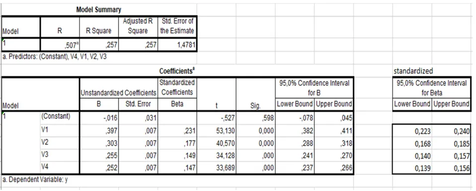
To illustrate how a PLS construct is an aggregator among its indicators and the rest of the model, but not an exact mediator (as it has no “disturbance” term), we can, for example, take a set of data simulated with the code of Annex. With this, a set of 50000 data was simulated with four predictor variables (“V1” to “V4”) with normal distribution and preset means (4.0; 3.0; 2.5 and 3.2), and with a standard deviation that equalled 1.0 in all four, and a correlation of 0.35 among them all. With V1, V2, V3 and V4, an unstandardised variable “y” was created as a linear combination with paths (0.4; 0.3; 0.25; 0.25) and a random error term so that the four predictors explained R2 = 0.25. In Figure 1 we observe the descriptives of the generated dataset. As the standard deviation of all the predictors equals 1, and that of variable “y” is 1.715, the standardised paths, which are those reported in programmes like SmarPLS, would respectively be 0.23; 0.17; 0.15, 0.15 (Betai unstad =(Sd Y/Sd Vi).betai std) (Fassott, Henseler & Coelho, 2016).
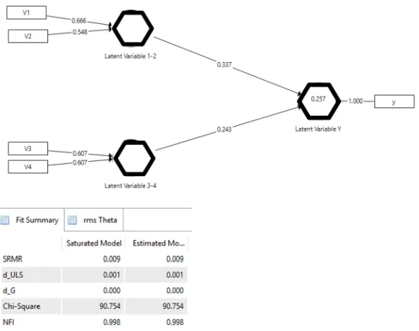
In Figure 2 we can see that the variables fit the design parameters. Figure 2 summarises the results of the analysis done with SPSS v22 and shows the standardised beta values and their confidence intervals. We can also see that the unstandardised coefficients coincide with those designed. Figure 3 shows that SmartPLS exactly reproduces the (standarised) regression results in both the estimated values and their confidence intervals because the contemplated model emulates multiple regression. Throughout this article, hexagons are used to represent based constructs (Bollen & Bauldry, 2011) (the origin of this notation apparently lies in the work by Grace and Bollen, 2008).
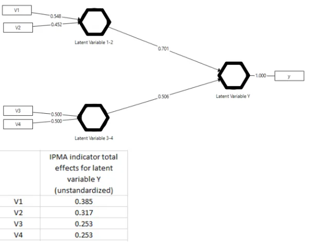
instance for V1, we can see that 0.666*0.337= 0.222, a value that comes very close to the original standardised path (0.231), but is not exactly the same. PLS does not report non-standardised values, but they can be calculated by starting with the descriptives of standard deviations or, more conveniently, the reports of the results using the IPMA of the SmartPLS procedure can be used for the total effects of the indicators of the model’s construct s (Figure 5)
Figure 1. The descriptives of the simulated dataset
Figure 3. The results of the model when emulating multiple regression with SmartPLS
Figure 5. “Unstandardised path coefficients” and “rescaled outer weights” with the IPMA procedure in SmartPLS
Between 2013 and 2016, several articles criticising the suitability of PLS as a scientific analysis method were published. These articles gave way to academic dispute, which led the Editor-in-Chief of some scientific journals in the operations management area to state that any article in which PLS was used as an analysis tool would quite likely be rejected by the Editor with no more ado. After reviewing the literature, all the objections made about PLS were answered in the responses that appear in other scientific journals (Cepeda-Carrion, Cegarra-Navarro & Cillo, 2019; Henseler, Dijkstra, Sarstedt, Ringle, Diamantopoulos, Straub et al., 2014; Sarstedt et al., 2016). In any case, an emphatic stance that denies any positive aspect of a technique or that blindly backs the exclusive appropriateness of a methodological approach apparently cannot be taken as good scientific practice, nor helps scientific disciplines to advance (Hair, Ringle & Sarstedt, 2012a; Kaufmann & Gaeckler, 2015).
After intense debate, what clearly came over was that the weaknesses of composite-based PLS-SEM do not mean that methods based on covariance (CB-SEM) are the best analysis tool for all cases (Kaufmann & Gaeckler, 2015). Indeed, biases emerge when PLS is used to estimate models in which only constructs exist as common factors, but also when CB-SEM is followed to estimate models in which constructs are composites. Therefore, it is necessary to select and carefully justify the method (PLS-SEM or CB-SEM) that is more suitable for the dataset to be analysed (Kaufmann & Gaeckler, 2015). If in doubt about the nature of constructs (if we are not clear about them being common factors or composites), it would be preferable to use PLS because it provides the least biased solutions (Sarstedt et al., 2016).
What all this debate has generated is a series of publications that attempt to systematise PLS being used as an analysis tool by means of usage guides or recommendations to make them more robust (Hair et al., 2019b; Henseler, Hubona & Ray, 2016a). Indeed, we believe it is interesting to summarise these guides.
3. Practical Guide. How Do We Avoid Frequent Errors In Articles Sent to Academic Journals?
3.1. Choice of Constructs
and, on the other hand, provides us with patterns to evaluate one of the criteria to be used to select the analysis procedure: CB-SEM or PLS-SEM.
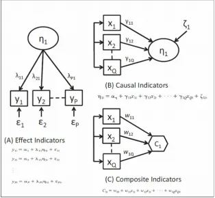
Items or indicators are variables with which we obtain a measure or observation during fieldwork, which helps us to estimate the parameters of latent/emergent variables (unobserved variables, but they represent a concept with an entity that is relevant for our analysis either because they naturally exist or are designed by people) (Grace & Bollen, 2008; Henseler, 2015, 2017a). To date, three types of indicators have been identified, which have given way to different measurement models in constructs (we will use constructs as a way to indistinctively refer to latent/emergent variables) (Figure 6): effect (or reflective) indicator (used in common factor constructs), causal indicator and composite indicator (it give rise to composite constructs) (Bollen & Bauldry, 2011; Grace & Bollen, 2008; Henseler, Ringle & Sarstedt, 2016b).
Figure 6. The three types of constructs (Bollen & Bauldry, 2011)
their indicators (Henseler et al., 2016b). This is why researchers are only interested in analysing the relation of this common variance with other parts of the model in the models they are present in. Indicators themselves are no object of interest, except for allowing parameters to be estimated because they are not considered levers on which to act and be used to modify constructs. Quite the opposite in fact as they are merely manifestations of the concept of interest (Bollen & Bauldry, 2011), and the variations of the existing construct, although we cannot measure it, are those that cause the values of indicators to vary. Attitudes, beliefs, intelligence test dimensions and personality traits are some paradigmatic examples of the social sciences constructs that tend to be modelled with effect indicators (Bollen & Bauldry, 2011). Generally speaking, the manifestations of the latent variables subject to the natural laws of any field (physics, mathematics, psychology, social sciences, etc.) tend to act as a suitable model with effect indicators (Henseler, 2015). For instance, anxiety of digitalisation (“computer anxiety”), understood as fears stemming from using computers, often takes an operational definition based on the effect indicators of the type “I avoid using computers for fear of making mistakes I can’t correct” or “I don’t feel happy about using computers” (Roberts & Thatcher, 2009).
Causal indicators, conversely, affect the latent variable (they cause it, and not vice versa). Hence causal indicators must have a conceptual unit or a shared meaning because they must all closely correspond to the definition selected for the unobserved construct (Bollen, 2011). We do not expect these indicators to be over-correlated, but no restriction is imposed in this case (Bollen & Bauldry, 2011; Roberts & Thatcher, 2009). At any rate, the construct exists in itself (even though it cannot be observed) (Grace & Bollen, 2008) and causal indicators compose a census, which is as complete as possible, of all the causes leading to it. This is why they are not interchangeable because, if one is suppressed, a considerable part of the causes is lost and the measurement error increases (Henseler, 2017a; Roberts & Thatcher, 2009). If, precisely, not all the causes are present, the construct will be measured with some error, represented by the term disturbance associated with the construct. In other words, the R2 of the construct will surely not be explained 100% by the indicators measured in research (Bollen, 2011), while the error term (disturbance) represents all the other causes not represented by the causal indicators included in the analysis (Roberts & Thatcher, 2009). If all these possible causes are contemplated with indicators, disturbance can be considered to equal zero (Diamantopoulos & Siguaw, 2006), in which case we could analyse the construct as if it were a composite (see later on). From a practical point of view, if the R2 of the latent construct explained by the indicators exceeds 0.26, the census of the indicators can be considered complete enough to contemplate the model with no disturbance (Diamantopoulos, 2006; Roberts & Thatcher, 2009). Moreover, as the construct itself exists, the weights of the indicators used to build the latent construct are relatively stable, despite the outcome variables associated with this construct changing (Bollen & Bauldry, 2011). For instance, the latent variable “exposure to stress” could take an operational definition based on causal indicators of these types, “changing jobs”, “getting married or divorced”, “suffering a serious disease” or “moving house”, which would act as a census of the possible causes for exposure to stress (Bollen & Bauldry, 2011). Each cause may have a distinct weight depending on its relative importance for producing stress. In this example, we may logically think that when someone suffers some of these causes (as it is not normal for everyone to suffer them all at once, the correlation among them would not be high), exposure to stress grows rather than someone being more predisposed to moving house, getting married, becoming ill and changing job (all at once) when stress grows. Indicators are the cause, and not the consequence, of the latent variable. So, it is foreseeable that the relative weight of the indicators is more or less stable because the intensity of the cause depends on its relation with the latent variable, and not with the constructs that the latent variable intends to explain.
indicator could modify the meaning of the construct. The emergent construct did not previously exist, but someone investigating creates/designs this construct and defines it as a linear combination of indicators (Whitt, 1986), and it is assumed by the restriction that R2 is 1; i.e., without the error term (Bollen, 2011; Grace & Bollen, 2008). Assigning the weight to the indicators of an emergent construct can be done in several ways, ranging from fixed weights (the unit or another value) to weights being estimated by some statistics procedure (correlations –Mode A- or regression coefficients –Mode B– are the commonest). If the weights of the indicators about the emergent construct are calculated with Mode B, they depend on the outcome variables (endogenous) included in the model, which we wish to explain. If the outcome variables are changed, it is quite likely that the weights of the composite indicators change (Bollen & Bauldry, 2011). In other words, if we take the composite indicators to be levers that we can move to achieve certain effects (effects that are assumed to be completely mediated by the emergent construct), the importance of these levers will depend on the effects that we wish to analyse. For instance, the relative weights of the components of a triple-A supply chain (adaptability, agility and alignment) may be different when they try to explain the competitive advantage than when they connect to the customer support and service level (Marin-Garcia, 2018). In the same way, if a profile of competences (emergent construct) is composed of indicators of creative behaviour, the manifestation of critical thought, technical knowledge about the job post and teamwork competency (Marin-Garcia, 2018), then it is foreseeable that the weights of these indicators differ when the competence profile is connected to explain the variance of a variable like “innovation results” from where it is connected to “organisational commitment” or to “piecework production capacity”. Generally, regardless of human designs being business practices, management models, performance indices, or even personal skills, as they are objects composed by elements, they may have suitable modelling with composite indicators, independently of other modellings being admitted. Thus, their data fit must be confirmed by the relevant analysis (Henseler, 2015; Henseler, 2017a).
3.2. Choosing the Estimation Technique
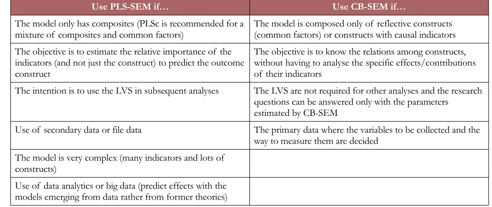
After defining which type of constructs appears in the model to be analysed, the next step consists in choosing the estimation technique that best fits the model (PLS-SEM, CB-SEM or others) (Sarstedt et al., 2016). Table 2 summarises the situations in which each analysis method would be recommendable (Dijkstra & Henseler, 2015a; Hair et al., 2017; Richter et al., 2016; Rigdon et al., 2016, 2017).
Use PLS-SEM if… Use CB-SEM if…
The model only has composites (PLSc is recommended for a
mixture of composites and common factors) The model is composed only of reflective constructs (common factors) or constructs with causal indicators The objective is to estimate the relative importance of the
indicators (and not just the construct) to predict the outcome construct
The objective is to know the relations among constructs, without having to analyse the specific effects/contributions of their indicators
The intention is to use the LVS in subsequent analyses The LVS are not required for other analyses and the research questions can be answered only with the parameters estimated by CB-SEM
Use of secondary data or file data The primary data where the variables to be collected and the way to measure them are decided
The model is very complex (many indicators and lots of constructs)
Use of data analytics or big data (predict effects with the models emerging from data rather from former theories)
3.3. Evaluating the Measurement Model
After making preliminary decisions, which have to be suitably informed and justified in the methodology section of any article to be sent to the JIEM Journal, two main analysis stages commence: evaluating the measurement model and evaluating the structure model.
The recommendations shown below only make sense when the chosen analysis method is PLS-SEM. Some recommendations have some parallelism when CB-SEM is used, but specific recommendations are based on the parameters or functionalities available in the specific computer programmes of PLS-SEM (SmartPLS 3 in particular (Ringle et al., 2015) or ADANCO (Henseler, 2017b)).
To evaluate the measurement model, we follow different steps depending on the nature of the construct’s indicators, which we define when specifying the measurement model. If constructs are common factors (effect indicators), Mode A (estimating the weight of constructs) should be selected. PLSc should be chosen in principle. However, a recent research work has suggested that it is preferable to use PLS in certain cases. Validation must follow four steps (Cepeda-Carrion et al., 2019; Hair et al., 2019b; Henseler, Ringle & Sarstedt, 2015; Voorhees, Brady, Calantone & Ramirez, 2016):
1. Item reliability: Loadings above 0.708
2. Internal consistency reliability: Composite reliability, Cronbach’s alpha values and Dijkstra and Henseler ρA above 0.70, but lower than 0.95
3. Convergent validity: Average variance extracted (AVE) over 0.50
4. Discriminant validity: The Heterotrait-monotrait (HTMT) value of correlations lower than 0.90 (the Fornell-Larcker criterion has been proven to not evaluate discriminant validity very well, especially if the loadings of all the indicators fall within a narrow range of values (0.65-0.85) (Henseler et al., 2015)) In those cases where all the items of a common factor construct can be considered interchangeable, re-specifying the measurement model by suppressing the indicators with worse psychometric properties is no serious problem (provided there are at least three retained indicators. However, having at least four is recommendable).
Constructs based on causal indicators cannot be estimated with PLS, unless disturbance is taken as zero (this is plausible when a complete census of indicators can be guaranteed or if the R2 of the construct is over 0.26 (Diamantopoulos, 2006; Roberts & Thatcher, 2009)). In this case, they will be dealt with like composites, otherwise they will be analysed with CB-SEM.
For emergent constructs based on composite indicators, unit weights can be estimated with a predefined value (if we wish to set the construct composition a priori), with Mode A (if not, PLSc is chosen because it would be estimated as a common factor with PLSc and Mode A) or with Mode B. Choosing Mode A or Mode B depends on if we require information about the effect of each indicator (Mode B) or only information about the effect of the construct (both Mode A and Mode B will do), correlations between indicators (Mode A if the correlation is high), sample size (Mode B with a small or medium sample size) and when the results are generalised beyond the sample (Mode A) (Becker, Rai & Rigdon, 2013a; Henseler et al., 2016a). Following four steps also is recommended for composites, but they differ from the steps followed for common factors (Cepeda-Carrion et al., 2019; Hair et al., 2019b; Ringle et al., 2018):
1. Convergent validity: (only when it has not been proven in previous research) the correlation exceeds 0.7 of the construct with an alternative measure of the same concept (a single-item, another already validated composite or a scale with effect indicators). Thus, the proposal put forward by Roberts and Thatcher (2009) can also be used. If the R2 of the composite is over 0.26, we may approach the causal indicator construct with a composite
2. Indicator collinearity: VIF values below 3
4. Relevance of indicator weights: the weights that come close to zero are of not much relevance, while the weights with absolute values above 1 tend to denote that a high collinearity exists among indicators or the sample is too small. It is also necessary to bear in mind that the maximum weight that an indicator may have (in Mode B) depends on the number of indicators (1/(n)^0.5 when there is no correlation among indicators). Thus, when the number increases, weights lower and the probability of them not being significant is greater. So, it is sometimes necessary to maintain non-significant indicators to maintain the conceptual definition or to make comparisons with other samples (compositional invariance)
We believe that there is no justification for eliminating a composite construct indicator, unless an items bank is being tested in a phase when measurement instruments are developed. If the scale is already validated or the indicator is included for some theoretical reason, it must be maintained in the model to not change the meaning of the construct, even if the weights and loadings of the indicator do not significantly differ from zero. An indicator whose weight comes close to zero will not affect the model’s calculations. It would no doubt penalise the statistical power of the analysis, but will not modify the LVS (because its value will be weighted by a weight that comes close to zero), nor will it affect the estimations of paths.
In the analysis requiring bootstraps, using at least 5000 samples is recommended, although 10000 will be ideal if the calculation time does not take too long (Ringle et al., 2018; Streukens & Leroi-Werelds, 2016).
To complete the measurement model’s validation, and to confirm that the appearance of the considered composites has been demonstrated, it is advisable to run a Confirmatory Composite Analysis (Henseler, 2017a; Schuberth et al., 2018a). To do so, it is necessary to check that the SRMR, d_ULG and d_G values of the saturated model are below either the 95% cut-off values or the 99% confidence interval of the bootstrap samples, in which case it is considered a good model (it cannot be rejected the hypothesis that the proposed model fits the data well).
Finally, before analysing the structural model, it is necessary to verify the measurement model’s invariance when possible groups exist to be compared (because data are grouped by some variable of interest for the research work or because different groups have been detected in the unobserved heterogeneity analysis). For each pair of groups, the Measurement Invariance of COmposite Models (MICOM) procedure can be followed with 5000 permutations or more, and by setting the significance level of the two-tailed test at 5% if there is no theoretical evidence for the sense of the difference among groups (Hair et al., 2018; Henseler et al., 2016a, 2016b). We must guarantee configural invariance by model design (step 1) using the same indicators for the constructs of each group. Then (step 2) compositional invariance is analysed to see if the composite have a correlation that is not significantly lower than 1 between each group; in other words, if the correlations of the original sample are above the 5% percentile of the correlations of the permutations (if the permutation p-values are over 0.05, then the weights of the composites’ indicators do not differ much among groups). If compositional invariance is met, in step 3 we check if the permutation-based confidence intervals of the differences of the means and the logarithms of the variance of the compared groups include the original values of the mean and logarithm of variance. Then we may consider full measurement invariance. Otherwise, we can consider that partial measurement invariance is met (a sufficient condition to make comparisons among the paths of groups when analysing the structure model using the same measurement model).
3.4. Evaluating the Structural Model
To evaluate the structural model, we must follow a six-step process(Cepeda-Carrion et al., 2019; Hair et al., 2019b; Shmueli, Ray, Velasquez-Estrada & Chatla, 2016):
1. Evaluate the collinearity among constructs. VIF values under 3 (if they go over 3, it might be worth creating HOC if the theoretical framework sustains this option)
cut-off must be modified depending on the constructs being considered, the model’s complexity and scientific disciplines
3. Blindfolding-based cross-validated redundancy measure Q2 (only for the endogenous constructs that are common factors). Values between 0 and 0.25 imply little predictive relevance, medium predictive relevance is denoted by values between 0.25 and 0.50, and predictive relevance is high if values exceed 0.5
4. The model’s out-of-sample predictive power (PLSpredict). By configuring with k-folds=10 and at least 10 repetitions. If Q2
predict is positive, the prediction error of the PLS-SEM model results is less than the prediction error based only on the mean of the values. The same happens when the values of the prediction errors (RMSE or MAE) are lower than PLS than with the LM benchmark.
5. Statistical significance of the paths’ coefficients: p-values of the T distribution are lower than 0.05 or the bootstrap confidence interval of paths does not include zero
6. Relevance of paths’ coefficients. The paths that come close to zero are poorly relevant. Alternatively, the value of f2 of each path can be analyzed, considering as cut values for low, moderate and high 0.02; 0.15 and 0.35 respectively
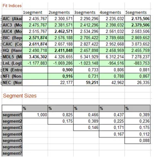
Unobserved heterogeneity must also be verified (if considering only one group for the analysis and estimating parameters are suitable). To do so, the PLS-SEM-based latent class methods can be used (Hair et al., 2019b; Hair et al., 2018; Ringle et al., 2018). Specifically, the FIMIX (finite mixture PLS) procedure allows us to detect how many non-homogeneous groups exist in the estimation of the parameters. With this objective, we must bear in mind:
• That the parameters of the fit indices, namely AIC, BIC, CAIC, HQ, MDL5 and LNL, suggest the number of segments for which the index takes a lower value. AIC tends to upwardly bias the recommendation of segments and MDL5 tends to downwardly bias. EN, NFI and NEC suggest the number of segments that make the index higher
• The number of cases ending up in each segment (Matthews, Sarstedt, Hair & Ringle, 2016; Sarstedt, Ringle & Hair, 2017)
It is useful to group the results of the different analyses in a table, highlight in bold the optimum values of each index and analyse the possible options, which are not normally convergent, by also including the distribution of cases (Figure 7). At the top we can see in each column the results of each analysis (the analysis are repeated by changing the number of segments to be estimated). Below we find the sizes of each segment. Checking several scenarios is recommended until most of the optimum fit index values coincide with one of them, or group sizes are so small that dividing sample into so many groups is not practical (loss of statistical power). In the example with an N with 183 cases, the fit indices suggest a scenario with a single segment or with a maximum of two segments. However, 82% of cases would go in one of the segments, which would leave the other with 33 cases, and could prove to be only a few to estimate the model with sufficient guarantees. As we can see, FIMIX provides information, but does not usually offer a single solution, and it is the researcher’s responsibility to justify the decisions made. For example, one option might be to isolate 17.5% of the cases and check that, when using only the subsample of the majority segment, it remains homogeneous, or if two similar sized subgroups appear, just as the solution of three initial segments may suggest. If more than one segment exists, the next step involves classifying data in this number of groups by predicted-oriented segmentation (POS) (Becker, Rai, Ringle & Völckner, 2013b).
Figure 7. Example of a summary of the FIMIX results, mainly solutions with 1, 2 or 3 segments
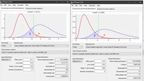
Finally, it is necessary to inform about the statistical power of the performed analyses and to check if sample size is sufficient for the magnitude of the found effects. The recommended statistical power value is 0.80 or higher with a significance level of 0.05 (Kaufmann & Gaeckler, 2015). If the two-stage procedure is followed to estimate LOC and then HOC, we must analyse the power in both stages and for all the endogenous constructs (normally the most unfavourable is that with a lower R2 and, at the same time, with more predictors). By starting with the R2 obtained in the PLS analysis, we can calculate f2=R2/(1- R2). With the value and number of predictors, we can estimate the power for the definite sample size with G*power (Faul, Erdfelder, Buchner & Lang, 2009) or with any other programme (e.g., the rutine pwr.f2.test in the pwr package of R (Champely, 2018)). This can also be done approximately using tables that provide us with the necessary sample to ensure suitable power (Hair et al., 2019a; Nitzl, 2016).
Figure 8. Procedure to calculate statistical power with G*power
The same results can be obtained with the pwr of R, as shown in Figure 10.
Figure 10. A priori calculation of statistical power with pwr
4. Conclusions
This article considers today’s PLS situation after intense academic debate of recent years, offers a summary that includes recommendations to conduct a PLS based research work reported with suitable information. We intend it to be used as a guide for researchers and possible authors who send works to JIEM. We also believe that it may be useful for any publication conducted with PLS, regardless of the journal it is sent to.
In this future research we will contemplate state of the theme relating to conducting research with PLS in operations management and to fit some of the cut-off values to the reality in the scientific field in this area (e.g., statistical power and the expected R2 levels).
Other relevant aspects that we have not been able to deal with in the present work in enough detail are:
• The need to present a guided example that respects all the report recommendations shown herein and that acts as a practical guide for authors.
• Does the specification or evaluation of the measurement model differ when first-order or second-order constructs are dealt with? What happens with the evaluation of HOC? Do they follow the same steps for LOC?
• How are the results of the constructs with indicators interpreted when they are measured with nominal measurement levels? If we wish to see the effect per variable category, an observed heterogeneity analysis is to be run (categorical/multigroup moderation). Using this construct as an explanatory variable might not make much sense, but using it as a adjusting variable may work. That is, it is used to fit the model, but analysing this construct is not of much interest and, instead, what happens with other constructs is interesting when the effect of this is included in the model.
• If the Confirmatory Composite Analysis approach (Henseler, 2017a; Schuberth et al., 2018a) is compatible with recent proposals made about the Confirmatory Tetrad Analysis (CTA) (Gudergan, Ringle, Wende & Will, 2008; Tabet, Lambie, G.W., Jahani, S., & Rasoolimanesh, 2019a, 2019b). This would allow us to analyse the measurement models of the operational definitions of latent variables; e.g., the skills of a job post that a worker masters, Total Production Maintenance (TPM)(Kareem & Amin, 2017; Marin-Garcia & Mateo-Martínez, 2013; Reyes, Alvarez, Martinez & Guaman, 2018), Lean Manufacturing, or the AMO model (Benet-Zepf, Marin-Garcia & Küster, 2018; Marin-Garcia & Martinez-Tomas, 2016). This would allow us to discern if they are “cultural” dimensions and if they exist themselves (and can, thus, explain organisational performances in the same way as personality exists and explains people’s conducts). Or perhaps it is a matter of artefacts, designed emergences that are created or acquired by summing capacities with different weights when explaining the results of interest.
We wish to look at these matters in more depth in subsequent publications.
Acknowledgements
We thank proffesors Dr. José Luís Roldán Salgueiro and Dr. Gabriel Cepeda-Carrion from Seville University for their remarks and the ideas they put forward via the PLS community in Spanish
Declaration of Conflicting Interests
The authors declared no potential conflicts of interest with respect to the research, authorship, and/or publication of this article.
Funding
The authors received no financial support for the research, authorship, and/or publication of this article.
References
Alfalla-Luque, R., Machuca, J.A.D., & Marin-Garcia, J.A. (2018). Triple-A and competitive advantage in supply chains: Empirical research in developed countries. International Journal of Production Economics, 203(September), 48-61. https://doi.org/10.1016/j.ijpe.2018.05.020
Ato, M., & Vallejo, G. (2011). Los efectos de terceras variables en la investigación psicológica. Anales de Psicología,
27(2), 550-561.
Avkiran, N.K. (2018). An in-depth discussion and illustration of partial least squares structural equation modeling in health care. Health Care Management Science, 21(3), 401-408. https://doi.org/10.1007/s10729-017-9393-7
Becker, J.M., Rai, A., & Rigdon, E.E. (2013a). Predictive validity and formative measurement in structural equation modeling: Embracing practical relevance. Paper presented at the Proceedings of the International Conference on
Information Systems. Milan, Italy.
Becker, J.M., Rai, A., Ringle, C.M., & Völckner, F. (2013b). Discovering unobserved heterogeneity in structural equation models to avert validity threats. MIS Quarterly: Management Information Systems, 37(3), 665-694.
https://doi.org/10.25300/MISQ/2013/37.3.01
Benet-Zepf, A., Marin-Garcia, J.A., & Küster, I. (2018). Clustering the mediators between the sales control systems and the sales performance using the amo model: A narrative systematic literature review. Intangible Capital, 14(3), 387-408. https://doi.org/10.3926/ic.1222
Bodoff, D., & Ho, S.Y. (2016). Partial least squares structural equation modeling approach for analyzing a model with a binary indicator as an endogenous variable. Communications of the Association for Information Systems, 28(23).
https://doi.org/10.17705/1CAIS.03823
Bollen, K.A. (2011). Evaluating effect, composite, and causal indicators in structural equation models. Mis Quarterly,
35(2), 359-372. https://doi.org/10.2307/23044047
Bollen, K.A., & Bauldry, S. (2011). Three cs in measurement models: Causal indicators, composite indicators, and covariates. Psychological Methods, 16(3), 265-284. https://doi.org/10.1037/a0024448
Callahan, J.L. (2018). The retrospective (im)moralization of self-plagiarism: Power interests in the social
construction of new norms for publishing. Organization, 25(3), 305-319. https://doi.org/10.1177/1350508417734926
Cepeda-Carrión, G., Cegarra-Navarro, J.G., & Cillo, V. (2019). Tips to use partial least squares structural equation modelling (pls-sem) in knowledge management. Journal of Knowledge Management, 23(1), 67-89.
https://doi.org/10.1108/JKM-05-2018-0322
Champely, S. (2018). Pwr: Basic functions for power analysis. R package version 1.2-2.
https://CRAN.R-project.org/package=pwr
Chin, W.W. (1998). Commentary: Issues and opinion on structural equation modeling. Mis Quarterly, VII-XVI.
Diamantopoulos, A. (2006). The error term in formative measurement models: Interpretation and modeling implications. Journal of modelling in management, 1(1), 7-17. https://doi.org/10.1108/17465660610667775
Diamantopoulos, A., & Siguaw, J.A. (2006). Formative versus reflective indicators in organizational measure development: A comparison and empirical illustration. British Journal of Management, 17(4), 263-282.
Dijkstra, T.K., & Henseler, J. (2015a). Consistent and asymptotically normal pls estimators for linear structural equations. Computational Statistics & Data Analysis, 81, 10-23. https://doi.org/10.1016/j.csda.2014.07.008
Dijkstra, T.K., & Henseler, J. (2015b). Consitent partial least squares path modeling. Mis Quarterly, 39(2), 297-316. do Valle, P.O., & Assaker, G. (2016). Using partial least squares structural equation modeling in tourism research: A
review of past research and recommendations for future applications. Journal of Travel Research, 55(6), 695-708.
https://doi.org/10.1177/0047287515569779
Duarte, P., & Amaro, S. (2018). Methods for modelling reflective-formative second order constructs in pls: An application to online travel shopping. Journal of Hospitality and Tourism Technology, 9(3), 295-313.
https://doi.org/10.1108/JHTT-09-2017-0092
Esposito-Vinzi, V., Chin, W.W., Henseler, J., & Wang, H. (2010). Handbook of partial least squares. Concepts, methods and applications. London: Springer.
Fassott, G., Henseler, J., & P.S.C. (2016). Testing moderating effects in pls path models with composite variables.
Industrial Management & Data Systems, 116(9), 1887-1900. https://doi.org/10.1108/IMDS-06-2016-0248
Faul, F., Erdfelder, E., Buchner, A., & Lang, A.G. (2009). Statistical power analyses using g*power 3.1: Tests for correlation and regression analyses. Behavior Research Methods, 41(4), 1149-1160.
https://doi.org/10.3758/BRM.41.4.1149
Felipe, C., Roldán, J., & Leal-Rodríguez, A. (2017). Impact of organizational culture values on organizational agility.
Sustainability, 9(12), 2354.
González De Dios, J. (2011). Checklist in systematic reviews and meta-analysis: The prisma statement, beyond the quorom. FMC Formacion Medica Continuada en Atencion Primaria, 18(3), 164-166.
https://doi.org/10.1016/S1134-2072(11)70060-3
Grace, J.B., & Bollen, K.A. (2008). Representing general theoretical concepts in structural equation models: The role of composite variables. Environmental and Ecological Statistics, 15(2), 191-213. https://doi.org/10.1007/s10651-007-0047-7
Gudergan, S.P., Ringle, C.M., Wende, S., & Will, A. (2008). Confirmatory tetrad analysis in pls path modeling.
Journal of Business Research, 61(12), 1238-1249.
Hair, J.F., Hult, G.T., Ringle, C.M., & Sarstedt, M. (2017). A primer on partial least squares structural equation modeling (pls-sem) (2nd ed.). Thousand Oaks: Sage.
Hair, J.F., Hult, G.T., Ringle, C.M., Sarstedt, M., Castillo-Apraiz, J., Cepeda Carrion, G. et al. (2019a). Manual de partial least squares structural equation modeling (pls-sem) (2nd ed.). Terrassa, Spain: OmniaScience:.
Hair, J.F., Ringle, C.M., & Sarstedt, M. (2012a). Partial least squares: The better approach to structural equation modeling? Long Range Planning, 45(5), 312-319. https://doi.org/10.1016/j.lrp.2012.09.011
Hair, J.F., Risher, J.J., Sarstedt, M., & Ringle, C.M. (2019b). When to use and how to report the results of pls-sem.
European Business Review, 31(1), 2-24. https://doi.org/10.1108/EBR-11-2018-0203
Hair, J.F., Sarstedt, M., Ringle, C.M., & Gudergan, S. (2018). Advanced issues in partial least squares structural equation modeling. Los Angeles: SAGE.
Hair, J.F., Sarstedt, M., Ringle, C.M., & Mena, J. (2012b). An assessment of the use of partial least squares structural equation modeling in marketing research. Journal of the Academy of Marketing Science, 40(3), 414-433.
Henseler, J. (2015). Is the whole more than the sum of its parts? On the interplay of marketing and design research: Initial lecture: Universiteit Twente
Henseler, J. (2017a). Bridging design and behavioral research with variance-based structural equation modeling.
Journal of Advertising, 46(1), 178-192. https://doi.org/10.1080/00913367.2017.1281780
Henseler, J., Dijkstra, T.K., Sarstedt, M., Ringle, C.M., Diamantopoulos, A., Straub, D. W. et al. (2014). Common beliefs and reality about pls: Comments on ronkko and evermann (2013). Organizational Research Methods, 17(2), 182-209. https://doi.org/10.1177/1094428114526928
Henseler, J., Hubona, G., & Ray, P.A. (2016a). Using pls path modeling in new technology research: Updated guidelines. Industrial Management & Data Systems, 116(1), 2-20. https://doi.org/10.1108/IMDS-09-2015-0382
Henseler, J., Ringle, C.M., & Sarstedt, M. (2015). A new criterion for assessing discriminant validity in variance-based structural equation modeling. Journal of the Academy of Marketing Science, 43(1), 115-135.
https://doi.org/10.1007/s11747-014-0403-8
Henseler, J., Ringle, C.M., & Sarstedt, M. (2016b). Testing measurement invariance of composites using partial least squares. International Marketing Review, 33(3), 405-431. https://doi.org/10.1108/IMR-09-2014-0304
Henseler, J., Ringle, C.M., & Sinkovics, R.R. (2009). The use of partial least squares path modeling in international marketing. In Sinkovics, R.R., & Pervez, N.G. (Eds.), Advances in international marketing (277-319). Bingley: Emerald Henseler, J., & Roldan, J.L. (2017). Coping with endogeneity in composite modeling. Paper presented at 8th Annual
Conference of the European Decision Sciences Institute. Granada, Spain.
Hock, C., Ringle, C.M., & Sarstedt, M. (2010). Management of multi-purpose stadiums: Importance and
performance measurement of service interfaces. International Journal of Services Technology and Management, 14(2-3), 188-207. https://doi.org/10.1504/IJSTM.2010.034327
Hult, G.T.M., Hair, J.F., Proksch, D., Sarstedt, M., Pinkwart, A., & Ringle, C.M. (2018). Addressing endogeneity in international marketing applications of partial least squares structural equation modeling. Journal of International Marketing, 26(3), 1-21. https://doi.org/10.1509/jim.17.0151
Jarvis, C.B., MacKenzie, S.B., & Podsakoff, P.M. (2003). A critical review of construct indicators and measurement model misspecification in marketing and consumer research. Journal of Consumer Research, 30(2), 199-218.
Kareem, J.A.H., & Amin, O. (2017). Ethical and psychological factors in 5s and total productive maintenance.
Journal of Industrial Engineering and Management-Jiem, 10(3), 444-475. https://doi.org/10.3926/jiem.2313
Kaufmann, L., & Gaeckler, J. (2015). A structured review of partial least squares in supply chain management research. Journal of Purchasing and Supply Management, 21(4), 259-272. https://doi.org/10.1016/j.pursup.2015.04.005
Kumar, D.S., & Purani, K. (2018). Model specification issues in pls-sem: Illustrating linear and non-linear models in hospitality services context. Journal of Hospitality and Tourism Technology, 9(3), 338-353.
https://doi.org/10.1108/JHTT-09-2017-0105
Latan, H. (2018). Pls path modeling in hospitality and tourism research: The golden age and days of future past
Applying partial least squares in tourism and hospitality researchedition: 1chapter: 4. Bingley: Emerald Publishing Limited Losilla, J.M., Oliveras, I., Marin-Garcia, J.A., & Vives, J. (2018). Three risk of bias tools lead to opposite conclusions
in observational research synthesis. Journal of Clinical Epidemiology, 101, 61-72.
https://doi.org/10.1016/j.jclinepi.2018.05.021
Marin-Garcia, J.A. (2018). Development and validation of spanish version of fincoda: An instrument for
self-assessment of innovation competence of workers or candidates for jobs. WPOM-Working Papers on Operations Management, 9(2), 182-215. https://doi.org/10.4995/wpom.v9i2.10800
Marin-García, Juan A., Alfalla-Luque, R. (2019). Protocol: How to deal with Partial Least Squares (PLS) research in Operations Management. A guide for sending papers to academic journals. WPOM-Working Papers on Operations Management, 10 (1), 29-69. https://doi.org/10.4995/wpom.v10i1.10802
Marin-Garcia, J.A., & Martinez-Tomas, J. (2016). Deconstructing amo framework: A systematic review. Intangible Capital, 12(4), 1040-1087. https://doi.org/10.3926/ic.838
Matthews, L.M., Sarstedt, M., Hair, J.F., & Ringle, C.M. (2016). Identifying and treating unobserved heterogeneity with fimix-pls: Part ii – a case study. European Business Review, 28(2), 208-224. https://doi.org/10.1108/EBR-09-2015-0095
Moher, D., Liberati, A., Tetzlaff, J., Altman, D.G., & The, P.G. (2009). Preferred reporting items for systematic reviews and meta-analyses: The prisma statement. PLoS Med, 6(7), e1000097.
https://doi.org/10.1371/journal.pmed.1000097
Moher, D., Shamseer, L., Clarke, M., Ghersi, D., Liberati, A., Petticrew, M. et al. (2016). Preferred reporting items for systematic review and meta-analysis protocols (prisma-p) 2015 statement. Revista Espanola de Nutricion Humana y Dietetica, 20(2), 148-160. https://doi.org/10.1186/2046-4053-4-1
Moher, D., Shamseer, L., Clarke, M., Ghersi, D., Liberati, A., Petticrew, M. et al. (2015). Preferred reporting items for systematic review and meta-analysis protocols (prisma-p) 2015 statement. Systematic Reviews, 4(1).
https://doi.org/10.1186/2046-4053-4-1
Muller, T., Schuberth, F., & Henseler, J. (2018). PLS path modeling - a confirmatory approach to study tourism technology and tourist behavior. Journal of Hospitality and Tourism Technology, 9(3), 249-266.
https://doi.org/10.1108/jhtt-09-2017-0106
Nitzl, C. (2016). The use of partial least squares structural equation modelling (pls-sem) in management accounting research: Directions for future theory development. Journal of Accounting Literature, 37, 19-35.
https://doi.org/10.1016/j.acclit.2016.09.003
Peng, D.X., & Lai, F. (2012). Using partial least squares in operations management research: A practical guideline and summary of past research. Journal of Operations Management, 30(6), 467-480.
Petter, S. (2018). Haters gonna hate: Pls and information systems research. SIGMIS Database, 49(2), 10-13.
https://doi.org/10.1145/3229335.3229337
Reyes, J., Alvarez, K., Martinez, A., & Guaman, J. (2018). Total productive maintenance for the sewing process in footwear. Journal of Industrial Engineering and Management-Jiem, 11(4), 814-822. https://doi.org/10.3926/jiem.2644
Richter, N.F., Cepeda, G., Roldán, J.L., & Ringle, C.M. (2016). European management research using partial least squares structural equation modeling (pls-sem). European Management Journal, 34(6), 589-597.
https://doi.org/10.1016/j.emj.2016.08.001
Rigdon, E., Sarstedt, M., & Ringle, C. (2017). On comparing results from cb-sem and pls-sem: Five perspectives and five recommendations. ZFP-Journal of Research and Management, 39(3), 4-16. https://doi.org/10.15358/0344-1369-2017-3-4
Rigdon, E.E. (2012). Rethinking partial least squares path modeling: In praise of simple methods. Long Range Planning, 45(5-6), 341-358. https://doi.org/10.1016/j.lrp.2012.09.010
Rigdon, E.E. (2014). Rethinking partial least squares path modeling: Breaking chains and forging ahead. Long Range Planning, 47(3), 161-167. https://doi.org/10.1016/j.lrp.2014.02.003
Rigdon, E.E. (2016). Choosing pls path modeling as analytical method in european management research: A realist perspective. European Management Journal, 34(6), 598-605. https://doi.org/10.1016/j.emj.2016.05.006
Ringle, C.M., & Sarstedt, M. (2016). Gain more insight from your pls-sem results: The importance-performance map analysis. Industrial Management & Data Systems, 116(9), 1865-1886. https://doi.org/10.1108/IMDS-10-2015-0449
Ringle, C.M., Sarstedt, M., Mitchell, R., & Gudergan, S.P. (2018). Partial least squares structural equation modeling in hrm research. The International Journal of Human Resource Management, 1-27.
https://doi.org/10.1080/09585192.2017.1416655
Ringle, C.M., Wende, S., & Becker, J.M. (2015). Smartpls 3. Boenningstedt: SmartPLS GmbH. Available at:
http://www.smartpls.com
Roberts, N., & Thatcher, J.B. (2009). Conceptualizing and testing formative constructs: Tutorial and annotated example. The DATA BASE for Advances in Information Systems, 4(3), 9-39.
Roldán, J.L., & Sánchez-Franco, M.J. (2012). Variance-based structural equation modeling: Guidelines for using partial least squares in information systems research. In Mora, M., Gelman, O., Steenkamp, A., & Raisinghani, M. (Eds.), Research methodologies, innovations and philosophies in software systems engineering and information systems (193-221). Hershey PA: IGI Global.
Sarstedt, M., Hair, J.F., Ringle, C.M., Thiele, K.O., & Gudergan, S.P. (2016). Estimation issues with pls and cbsem: Where the bias lies! Journal of Business Research, 69(10), 3998-4010. https://doi.org/10.1016/j.jbusres.2016.06.007
Sarstedt, M., Ringle, C.M., & Hair, J.F. (2017). Treating unobserved heterogeneity in pls-sem: A multi-method approach. In H. Latan & R. Noonan (Eds.), Partial least squares path modeling: Basic concepts, methodological issues and applications (197-217). Cham: Springer International Publishing
Schuberth, F., Henseler, J., & Dijkstra, T.K. (2018a). Confirmatory composite analysis. Frontiers in Psychology, 9(2541), 1-14. https://doi.org/10.3389/fpsyg.2018.02541
Schuberth, F., Henseler, J., & Dijkstra, T.K. (2018b). Partial least squares path modeling using ordinal categorical indicators. Quality & Quantity, 52(1), 9-35. https://doi.org/10.1007/s11135-016-0401-7
Sharma, P.N., Sarstedt, M., Shmueli, G., Kim, K.H., & Thiele, K.O. (2019). Pls-based model selection: The role of alternative explanations in information systems research. Journal of the Association for Information Systems, in press. Shmueli, G., Ray, S., Velasquez-Estrada, J.M., & Chatla, S.B. (2016). The elephant in the room: Predictive
performance of pls models. Journal of Business Research, 69(10), 4552-4564.
https://doi.org/10.1016/j.jbusres.2016.03.049
Streukens, S., & Leroi-Werelds, S. (2016). Bootstrapping and pls-sem: A step-by-step guide to get more out of your bootstrap results. European Management Journal, 34(6), 618-632. https://doi.org/10.1016/j.emj.2016.06.003
Tabet, S.M., Lambie, G.W., Jahani, S., & Rasoolimanesh, S.M. (2019a). An analysis of the world health organization disability assessment schedule 2.0 measurement model using partial least squares–structural equation modeling.
Assessment, 1073191119834653. https://doi.org/10.1177/1073191119834653
Tabet, S.M., Lambie, G.W., Jahani, S., & Rasoolimanesh, S.M. (2019b). The factor structure of outcome questionnaire–45.2 scores using confirmatory tetrad analysis–partial least squares. Journal of Psychoeducational Assessment, 0734282919842035. https://doi.org/10.1177/0734282919842035
Urbach, N., & Ahleman, F. (2010). Structural equation modeling in information systems research using partial least squares. Journal of Information Technology Theory and Application, 11(2), 1-39.
Urrútia, G., & Bonfill, X. (2010). Prisma declaration: A proposal to improve the publication of systematic reviews and meta-analyses. Medicina Clinica, 135(11), 507-511. https://doi.org/:10.1016/j.medcli.2010.01.015
Urrútia, G., & Bonfilll, X. (2013). The prisma statement: A step in the improvement of the publications of the revista española de salud pública. Revista Española de Salud Pública, 87(2), 99-102.
https://doi.org/10.4321/S1135-57272013000200001
Usakli, A., & Kucukergin, K.G. (2018). Using partial least squares structural equation modeling in hospitality and tourism: Do researchers follow practical guidelines? International Journal of Contemporary Hospitality Management,
30(11), 3462-3512. https://doi.org/10.1108/IJCHM-11-2017-0753
Voorhees, C., Brady, M., Calantone, R., & Ramirez, E. (2016). Discriminant validity testing in marketing: An analysis, causes for concern, and proposed remedies. Journal of the Academy of Marketing Science, 44(1), 119-134.
Welch, V., Petticrew, M., Petkovic, J., Moher, D., Waters, E., White, H. et al. (2015). Extending the prisma statement to equity-focused systematic reviews (prisma-e 2012): Explanation and elaboration. International Journal for Equity in Health, 14(1). https://doi.org/10.1186/s12939-015-0219-2
Welch, V., Petticrew, M., Petkovic, J., Moher, D., Waters, E., White, H. et al. (2016a). Extending the prisma statement to equity-focused systematic reviews (prisma-e 2012): Explanation and elaboration. Journal of Clinical Epidemiology,
70, 68-89. https://doi.org/10.1016/j.jclinepi.2015.09.001
Welch, V., Petticrew, M., Petkovic, J., Moher, D., Waters, E., White, H., et al. (2016b). Extending the prisma statement to equity-focused systematic reviews (prisma-e 2012): Explanation and elaboration. Journal of Development Effectiveness, 8(2), 287-324. https://doi.org/10.1080/19439342.2015.1113196
Welch, V., Petticrew, M., Tugwell, P., Moher, D., O’Neill, J., Waters, E. et al. (2013). Prisma-equity 2012 extension: Reporting guidelines for systematic reviews with a focus on health equity. Revista Panamericana de Salud Publica/Pan American Journal of Public Health, 34(1), 60-67.
Welch, V., Petticrew, M., Tugwell, P., Moher, D., O’Neill, J., Waters, E. et al. (2012). Prisma-equity 2012 extension: Reporting guidelines for systematic reviews with a focus on health equity. PLoS Medicine, 9(10).
https://doi.org/10.1371/journal.pmed.1001333
Whitt, H.P. (1986). The sheaf coefficient: A simplified and expanded approach. Social Science Research, 15(2), 174-189. https://doi.org/10.1016/0049-089X(86)90014-1
Annex
Code R for data simulation
Adapted from:
• https://stackoverflow.com/questions/46808859/simulating-multiple-regression-data-with-fixed-r2-how-to-incorporate-correlated
• https://www.google.com/url?
sa=t&rct=j&q=&esrc=s&source=web&cd=6&ved=2ahUKEwj3mvrEgufgAhXfA2MBHZ2wBkgQFjAFegQIBhA C&url=http%3A%2F%2Fwww.statpower.net%2FContent%2F310%2FThe%2520Laws%2520of%2520Linear %2520Combination.pdf&usg=AOvVaw0gWD3ZSjrovJwnR5-FPV59
• Fassott, G., Henseler, J., & P.S, C. (2016). Testing moderating effects in pls path models with composite variables. Industrial Management & Data Systems, 116(9), 1887-1900. https://doi.org/10.1108/IMDS-06-2016-0248
# Specify population means and standard deviation of four predictor variables that is sampled from std<-c(1,1,1,1) #Standard deviations values desired by design for V1 to V4
var<-std^2
mu<-c(4,3,2.5,3.2) #mean values desired by design for V1 to V4
corxx<-0.35 #correlations desired by design between V1 to V4 (all equal) sigma.1 <- matrix(c(1,corxx,corxx,corxx,
corxx,1,corxx,corxx, corxx,corxx,1,corxx,
corxx,corxx,corxx,1),nrow=4,ncol=4) mu.1 <- rep(0,4)
# Specify sample size, true regression coefficients, and explained variance n.obs <- 500 # 500000 recommended to avoid sampling error problems
beta <- c(0.4, 0.3, 0.25, 0.25) #unstandardized Beta coefficients for lineal combination of V1 to V4 to create y (unstandardized)
r2 <- 0.25 #
# Create sample with four predictor variables library(MASS)
sample1 <- as.data.frame(mvrnorm(n = n.obs, mu.1, sigma.1, empirical=FALSE)) 'standardized Vi variables'
apply(sample1, 2, mean) apply(sample1, 2, sd)
# dataframe with independent values without standardization (y variable it is not standardized. Mean= intercept and variance depends on equation above sample1$y)
sample2<-as.data.frame(sample1) sample2$V1<-sample2$V1*std[1]+mu[1] sample2$V2<-sample2$V2*std[2]+mu[2] sample2$V3<-sample2$V3*std[3]+mu[3] sample2$V4<-sample2$V4*std[4]+mu[4] # Add error variable based on desired r2
var.epsilon <- (beta[1]^2+beta[2]^2+beta[3]^2+beta[4]^2+corxx)*((1 - r2)/r2) #original si todas las corr son iguales
sample1$epsilon <- rnorm(n.obs, sd=sqrt(var.epsilon)) # Add y variable based on true coefficients and desired r2
sample2$y <- intercept + beta[1]*sample2$V1 + beta[2]*sample2$V2 + beta[3]*sample2$V3 + beta[4]*sample2$V4 + sample1$epsilon
'variables unstandardized' apply(sample2, 2, mean) apply(sample2, 2, sd) # Inspect model
summary(lm(scale(y)~scale(V1)+scale(V2)+scale(V3)+scale(V4), data=sample2)) summary(lm(y~V1+V2+V3+V4, data=sample2))
cor(sample1) cor(sample2) # Write CSV in R
write.csv(sample2, file = "MyData500.csv",row.names=FALSE, na="-999"
Journal of Industrial Engineering and Management, 2019 (www.jiem.org)
Article’s contents are provided on an Attribution-Non Commercial 4.0 Creative commons International License. Readers are allowed to copy, distribute and communicate article’s contents, provided the author’s and Journal of Industrial Engineering and