Department of Mathematics
Ph.D. in Mathematics Ciclo XXV
On structure and decoding of Hermitian
codes
Chiara Marcolla
Supervisor: Prof. Massimiliano Sala
Head of PhD School: Prof. Alberto Valli
Department of Mathematics
Ph.D. in Mathematics Ciclo XXV
On structure and decoding of Hermitian
codes
Ph.D.Thesis of:
Chiara Marcolla
Supervisor:
Prof. Massimiliano Sala
Head of PhD School:
Prof. Alberto Valli
I Preliminaries
1
1 Coding Theory 3
1.1 An overview on error correcting codes . . . 3
1.2 Linear codes . . . 4
1.2.1 Basic denitions . . . 4
1.2.2 Decoding linear codes . . . 6
1.2.3 Probability of the Undetected Error . . . 8
1.3 Cyclic codes . . . 9
1.3.1 An algebraic correspondence . . . 9
1.3.2 Encoding and decoding with cyclic codes . . . 12
2 Introduction to Gröbner bases 15 2.1 Monomial ordering . . . 15
2.2 Basic notions about ideals and Gröbner bases . . . 18
2.3 Elimination Theory . . . 24
3 Hermitian and Norm-Trace curves 27 3.1 Known facts on Norm-Trace curve and Hermitian curve . . . 27
3.2 Intersection between the Hermitian curve H and a line . . . 28
3.3 Automorphisms of Hermitian curve . . . 29
3.4 Automorphisms of Norm-Trace curve . . . 30
4 Ane-variety codes 31 4.1 Anevariety codes . . . 31
4.2 Norm-Trace codes and Hermitian codes . . . 32
4.2.1 First results on words of given weight . . . 33
4.3 The approach by Fitzgerald and Lax to decoding the ane-variety code 34 4.4 Base notion for decoding using our method . . . 35
4.4.1 Stratied ideals . . . 35
4.4.2 Root multiplicities and Hasse derivative . . . 37
5.1 Numerical semigroups . . . 41
5.2 Analysing Hermitian codes using numerical semigroups . . . 42
5.3 Phases intersections . . . 46
II Main Results
53
6 Intersections between the Hermitian curve H and parabolas 55 6.1 Odd characteristic . . . 586.1.1 Intersection betweenH and y=ax2+c . . . . 58
6.1.2 Intersection betweenH and y=ax2+bx+c . . . . 62
6.2 Even characteristic . . . 68
7 Small-weight codewords of Hermitian codes 71 7.1 Corner codes and edge codes . . . 71
7.2 First results for the rst phase . . . 72
7.3 Minimum-weight codewords . . . 74
7.4 Second-weight codewords . . . 78
7.5 The complete investigation for d= 3,4. . . 82
7.6 On the geometry of small weight codewords of AG codes . . . 87
8 Decoding of ane-variety codes 95 8.1 Decoding with ghost points . . . 96
8.2 Weak locator polynomials . . . 101
8.3 Results on some zerodimensional ideals . . . 110
8.4 Proof of Proposition 8.3.13 . . . 118
8.4.1 Preliminaries of proof . . . 118
8.4.2 Sketch of proof . . . 120
8.4.3 First part of the proof . . . 121
8.4.4 Second part of proof . . . 122
8.4.5 Third part of the proof . . . 125
8.5 Multi-dimensional general error locator polynomials . . . 127
8.6 Stued ideals . . . 131
8.7 Families of anevariety codes . . . 135
8.7.1 SDG curves . . . 135
8.7.2 SDG surfaces I . . . 136
8.7.3 SDG surfaces II . . . 137
III Programs and Computations
141
9 Hermitian curve and Hermitian code 143
9.1 MAGMA programs to compute intersection between H and parabolas. 143
9.2 MAGMA programs to compute the number of minimum-weight words of Hermitian code. . . 148 9.3 Singular programs to compute the number of words of weight d+ 1. . 151
10 Decoding anevariety code 155
10.1 Singular programs to nd weak locators. . . 155 10.2 Singular programs to nd the locators. . . 158
Given a linear code, it is important both to identify fast decoding algorithms and to estimate the rst terms of its weight distribution. Ecient decoding algorithms allow the exploitation of the code in practical situations, while the knowledge of the number of small-weight codewords allows to estimate its decoding performance. For ane-variety codes and its subclass formed by Hermitian codes, both problems are as yet unsolved. We investigate both and provide some solutions for special cases of interest.
The rst problem is faced with use of the theory of Gröbner bases for zero-dimensional ideals.
The second problem deals in particular with small-weight codewords of high-rate Hermitian codes. We determine them by studying some geometrical properties of the Hermitian curve, specically the intersection number of the curve with lines and parabolas.
This thesis is divided in two parts.
The rst part contains preliminaries and known results except for some sections that contain original results, namely Section 3.4 where we nd some automorphisms of Norm-Trace curve and Subsection 4.2.1 which is devoted to nd a system that permits us to compute the number of words of a given weight. Finally in Section 5.3 we revisit the phases of Hermitian codes proposed by [HvLP98].
Known results include basic theory and notations of linear codes ([AE09],[HP03], [MS77]) and of Gröbner bases ([CLO07], [ST09]). Some material comes from the lec-ture notes of the course Coding Theory leclec-tured by M. Sala and written by E. Bellini, D. Frapporti, O. Geil, M. Piva, M. Sala). In Chapter 4 we dene the most important objects of this thesis, that is, the Ane-variety codes and Hermitian codes, explain the classical decoding and provide some preliminary results for our decoding method.
In Chapter 6 the main result is Theorem 6.0.1, where we provide a complete classication of intersections between H and any parabola y = ax2 +bx +c (a6= 0). The proof is divided in three main parts. In the rst part of Chapter 6 we lay down some preliminary lemmas and we skecth our proving argument, that is, the use of the authomorphism group forH. In Section 6.1 we deal with the
odd-characteristic case and in Section 6.2 we deal with the even-characteristic case.
In the beginning of Chapter 7 we analyse in depth the rst-phase Hermitian codes (that is, codes such that d ≤ q). We give our algebraic
characteriza-tion in Seccharacteriza-tion 7.2 and we use these results to completely classify geometrically the minimum-weight codewords for all rst-phase codes in Section 7.3. In Sec-tion 7.4 we can count some special conguraSec-tions of second-weight codewords for any rst-phase code and nally in Section 7.5 we can count the exact number of second-weight codewords for the special case whend= 3,4.
In Chapter 8 we generalize the general error locator polynomials (that are poly-nomials introduced in [OS05] to decode cyclic codes) to cover also the multi-dimensional case and hence the ane-variety case. This chapter contains the following sections.
- In Section 8.1 we introduce the notion of ghost points, which are points added to the variety to play the role of non-valid error locations.
- Using the denition of ghost point, in Section 8.2 we can dene a rst generalization of general error locator polynomials to the multivariate case (Denition 8.2.5), which provides a rst decoding strategy. We also in-troduce evaluator polynomials (Denition 8.2.6) that permits a second strategy.
sition describes some features of the Gröbner basis of (the elimination ideals of) a zero-dimensional radical idealJ. The proof is constructive and
relies on iterated applications of some versions of the Buchberger-Möller algorithm.
- Unfortunately, result in the multidimensional case, Proposition 8.3.13, is not as strong as our result in the one-variable case, Proposition 4.4.3. In Section 8.5, it does allow us to prove the existence of our rst generalization of locators in Theorem 8.5.1, but we show that better locators can be found, as in Denition 8.5.2. We discuss with examples a new decoding strategy by applying these locators, but for the moment we are unable to prove their existence, since they use multiplicities. This will be done in the next section.
- In Section 8.6 we develop the theory for generalizing stratied ideals to the multivariate case with multiplicities.
As usual, we are interested in suitable Gröbner bases of elimination ideals of some zero-dimensional ideals. First, we introduce the notion of stued ideals (Denition 8.6.1), which basically means that the roots of some polynomials in these Gröbner bases have the expected multiplicity. We give a constructive method (stung) to obtain stued ideals from special classes of ideals (in particular, radical ideals will do). Our main results here are Theorem 8.6.4, that ensures that the desired shape of our Gröbner bases is unchanged under stung, and Theorem 8.6.6, that ensures the existence of our sought-after locators (in our Gröbner bases).
- In Section 8.7 we compute some examples from dierent families of ane-variety codes. In particular, we formally determine the shape for multi-variate locator polynomials in the Hermitian case, for anyq ≥2 andt = 2 (Theorem 8.7.3), both in our weaker version and in our stronger version. In Chapter 9 we show how we computed specic examples and tested
experi-mentally all our counting results.
In this chapter we summarize denitions and known results from [AE09, HP03, MS77].
We denote by Fq the eld with q elements, where q is a power of a prime, and
by n ≥ 1 a natural number. Let (Fq)n be the vector space of dimension n over Fq.
From now on, we denote byKany (not necessarily nite) eld and by Kits algebraic closure.
1.1 An overview on error correcting codes
In 1948 Claude Shannon published a paper, A mathematical theory of commu-nication [Sha48], that was the beginning of Coding Theory. In this paper Shannon dened a numberQ called the capacity of the channel and proved that for any given
degree of noise contamination of a communication channel, it is possible a communi-cation nearly error-free up to Q.
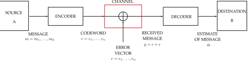
This result guarantees that any data can be encoded before transmission so that the altered data can be decoded to the specied degree of accuracy. Hence the codes were invented to correct the errors that occur during the transmission. The basic idea of coding theory consists of adding some kind of redundancy to the message m which
the information source A wants to send to a destination B.
In the Figure 1.1 the messagem is encoded by the encoder into a codeword cand
CHANNEL
SOURCE A
DESTINATION B
MESSAGE CODEWORD RECEIVED ESTIMATE
MESSAGE OF MESSAGE ERROR
VECTOR m=m1, . . . , mk c=c1, . . . , cn
e=e1, . . . , en
y=c+e mˆ
ENCODER DECODER
Figure 1.1: A communication schema
error vector. Finally the vector y is decoded using the decoder, but only if the
oc-curred errors are not too many (in a sense that will be clear later), the receiver is able to recover the original message m.
In the next sections we will describe some basic concepts about coding theory considering the coding procedure as a linear function between vector spaces.
1.2 Linear codes
1.2.1 Basic denitionsLinear codes are widely studied because of their algebraic structure, which makes them easier to describe than non-linear codes.
Denition 1.2.1. Let k, n ∈ N such that 1 ≤ k ≤ n. A vector subspace of (Fq)n of
dimension k is a linear codeC over Fq with length n and dimension k. An element
of C is called a word of C.
We indicate by [n, k]q a linear code over Fq with length n and dimension k and
we call binary code a code over F2.
Note that if C is a linear code[n, k]q, thanC has qk codewords.
Denition 1.2.2. If C is an [n, k]q code, then any k×n matrix G whose rows form
a basis for C is called a generator matrix for C.
In general there are many generator matrices for a code. For any set of k
inde-pendent columns of a generator matrixG, the corresponding set of coordinates forms
an information set for C. The remaining r =n−k coordinates forms a redundancy
set and r is called the redundancy of C. If the rst k coordinates form an information set, thenC has a unique generator matrixG=Ik |A
, whereIk is thek×k identity
matrix. G is called a generator matrix in standard form.
Thanks to this algebraic description, to encode a message m ∈ (Fq)k into the
word c∈ (Fq)n, it is sucient to perform the matrix multiplication mG =c. When
the generator matrix is in standard form [Ik | A], m is encoded in mG = (m, mA),
where(x, y)denote the vector obtained by the concatenation of xand y. In this case
the message m is formed by the rst k components of the associated word. For this
reason, the set formed by the rst k columns of G is called information set and this
Denition 1.2.3. If C is an [n, k]q code, its dual code C⊥ is the set of vectors
orthogonal to all words of C:
C⊥={v ∈(Fq)n|v·c= 0,∀c∈C}.
Thus C⊥ is an [n, n−k]q code.
A generator matrix of C⊥ is called parity-check matrix ofC.
Denition 1.2.4. A parity-check matrix H for an [n, k]q code C is a generator
matrix (n−k)×n for C⊥.
It is easy to see that C may be expressed as the null space of a parity-check
matrix H, that is,
∀x∈(Fq)n, HxT = 0 ⇐⇒ x∈C.
Theorem 1.2.5. If G = Ik | A
is a generator matrix for the [n, k]q code C in
standard form, then H =
AT |I n−k
is a parity check matrix for C
Proof. See Theorem 1.2.1 of [HP03].
For any two vectors x, y ∈ (Fq)n, we dene the (Hamming) distance d(x, y)
be-tween x and y as the number of coordinates in whichx and y dier.
Whereas, the (Hamming) weight w(x) of a vector x ∈ (Fq)n is the number of its
nonzero coordinates, that is,
w(x) = d(x,0).
Denition 1.2.6. The distance of a code C is the smallest distance between
dis-tinct words, that is,
d(C) = min{d(ci, cj)|ci, cj ∈C, ci 6=cj}.
If we know the distance d=d(C)of an [n, k]q code, then we can refer to the code
as an [n, k, d]q code.
It is simple to prove that following proposition. Proposition 1.2.7. Let C be a [n, k, d]q code, then
d(C) = min{w(c)|c ∈ C, c6= 0}.
Denition 1.2.8. Let C be an [n, k, d]q code and let Ai be the number of codewords
having weight i. The weight distribution of C is the sequence {Ai} with 1≤i≤n.
If for any i, Ai =An−i, then we have a symmetric weight distribution.
Proposition 1.2.9. Let C be an [n, k, d]q code and let H be a parity-check matrix
of C. If H has w linearly dependent columns, then exists a codeword in C of weight
less than or equal to w. As a consequence, if any subset of r columns of H is linearly
independent, then d(C)≥r+ 1.
An immediate consequence of the previous proposition is an upper bound on the distance of a code in terms of the length and the dimension.
Proposition 1.2.10 (Singleton Bound). Let C be an [n, k, d]q code, then
d≤n−k+ 1.
A code achieving this bound is called maximum distance separable (MDS). Finally, we dene a subcode of a code C as a subspace ofC.
1.2.2 Decoding linear codes
The distance of a code C is important to determine both the error correction
capability of C, that is, the number of errors that the code can correct and its error
detection capability, that is, the number of errors that the code can detect. In fact, we can see the noise as a perturbation that moves a word into some other vector. If the distance between the words is large, there is a low probability that the noise can move a codeword near to another one. To be more precise, we have the following theorem.
Theorem 1.2.11. Let C be an [n, k, d]q code, then C has detection capability d−1
and it has correction capability t=bd−1 2 c.
Proof. See Theorem 1.11.4 of [HP03] or Theorem 2 of 3 of [MS77, 1].
Let c∈C be the word transmitted and let y∈(Fq)n be the vector received, then
e=y−cis the error vector. If we apply the parity-check matrix H toy, we get: HyT =H(c+e)T =HeT =s.
Denition 1.2.12. The elements in (Fq)n−k, s =HyT, are called syndromes. We
say that s is the syndrome corresponding to y.
Note that if we transmit another word and the same error e occurs, we get the
same syndrome. So the syndrome does not depend on the specic word sent, but only on the occurred error e.
Note that(Fq)n can be partitioned into qn−k cosets of size qk.
Two vectors a, b ∈ (Fq)n belong to the same coset if and only if a −b ∈ C. The
following fact is just a reformulation of our arguments.
Theorem 1.2.13. Let C be an [n, k, d]q code. Two vectors a, b ∈ (Fq)n are in the
same coset if and only if they have the same syndrome.
Proof. Leta, b∈(Fq)n. Thena, b belong to the same coset if and only if
a−b ∈ C ⇐⇒ H(a−b)T = 0 ⇐⇒ HaT =HbT.
Denition 1.2.14. Let C be an [n, k, d]q code. For any coset a+C and any vector
v ∈a+C, we say that v is a coset leader if it is an element of minimum weight in
the coset.
Denition 1.2.15. Ifs is a syndrome corresponding to an erroreof weight w(e)≤t,
then we say that s is a correctable syndrome and e a correctable vector error.
Theorem 1.2.16 (Correctable syndrome). If no more than t errors occurred (i.e.
w(e)≤t), then there exists only one errorecorresponding to the correctable syndrome s=He and e is the unique coset leader of e+C.
Proof. See Corollary 1.11.3 of [HP03]
We are ready to describe the decoding algorithm of linear codes, that is the de-coding using standard array. The standard array is a matrix that contains the 2n vectors of (Fq)n ordered by coset. Then the complexity of the decoding procedure is
exponential in terms of memory occupancy. The decoding procedure is the following.
1. After receiving a vector y∈(Fq)n, compute the syndromes =HyT.
2. Find z, a coset leader of the corresponding coset.
This is equivalent to nding a vectoreof smallest weight in the coset containing y such that y−e∈C.
3. The decoded word is c=y−z.
4. Recover the message m from c (in case of systematic encoding m consists of
rst k components ofc).
1.2.3 Probability of the Undetected Error
When decoding using the standard array, the error vector echosen by the decoder
is always one of the coset leaders. The decoding is correct if and only if the true error vector is the coset leader. That is, if w(e)> t, then the decoder may make an error
and the output is another codeword. The probability that the decoder output is the wrong codeword is called Probability of the Undetected Error (PUE) or word error rate.
We will dene the PUE in a q-ary symmetric channel. That is,
Denition 1.2.17. A q-ary symmetric channel (SC) is a channel which has the following properties:
1. the component of a transmitted word (that we call symbol) can be changed only to another element of Fq.
2. The probability that a symbol becomes another one is the same for all symbols. 3. The probability that a symbol changes during the transmission does not depend
on its position.
4. If the i-th component is changed, then this fact does not aect the probability of
change for the j-th components.
To these channel properties it is usually added a source property, that is, 5. all words are equally likely to be transmitted.
Obviously, the q-ary SC is a model that rarely can describe real channels, but it
permits a simpler construction of the theory. Now we are going to see in which way. Letpbe the probability that the symbol1become0or vice-versa where1≤p <1/q.
Suppose that during the transmission occurs an errore. The probability thate is the
vector v ∈(Fq)n of weight i is
P rob{e =v}=pi(1−p)n−i. (1.1)
Hence, if the code C has weight distribution{Ai} with 0≤i≤n, then by (1.1)
P U E=
n
X
i=1
Aipi(1−p)n−i.
Note that if p is very low, then the PUE is more inuenced by the small weight
1.3 Cyclic codes
1.3.1 An algebraic correspondence
Denition 1.3.1. An [n, k, d]q linear codeC is a cyclic code if the cyclic shift of a
word is also a word, that is,
(c0, . . . , cn−1)∈C =⇒ (cn−1, c0, . . . , cn−2)∈C.
A powerful instrument to describe algebraic properties of cyclic codes is to rep-resent codewords in polynomial form. Detail can be found in Chapter 4 of [HP03]. Here we report an informal introduction of some tools that we will use in Section 2.2.
Let Fq[x] be a polynomial ring. For any f ∈Fq[x] we denote
hfi={f g|g ∈Fq[x]}
and we say thathfiis an ideal. We construct a bijective correspondence between the
vectorsc= (c0, . . . , cn−1)of(Fq)nand the polynomialsc(x) = c0+c1x+· · ·+cn−1xn−1 inFq[x] of degree at most n−1.
Note that if c(x) is a word, then the shift to the right of c(x) is xc(x) mod xn−1. This suggests that the words of cyclic codes can be represented as polynomials in a residue class ringR=Fq[x]/I, whereI is the idealI =hxn−1i. So we can identifyC
with a subset ofRand thus, with a slight abuse of notation, we can multiply elements
of C with polynomials moduloxn−1
Knowing that xi·c∈C for any c∈C, it is simple to prove the following theorem.
Theorem 1.3.2. Let C be an [n, k, d]q code. Then C is cyclic if and only if C is an
ideal of R.
Let C be an [n, k, d]q cyclic code. It is easy to prove (see Theorem 4.2.1 and
Corollary 4.2.2 of [HP03]) that there exists a unique monic polynomial g of minimal
degree that generates C as an ideal of R. Moreover,
if C =hgi =⇒ g divides xn−1in Fq[x] and its degree is deg(g) = n−k.
We callg the generator polynomial of C.
A generator matrix can easily be given by using the coecients of the generator polynomial g =Pn−k
i=0 gixi:
G= g xg ...
xkg
=
g0 g1 . . . gn−k 0 . . . 0
0 g0 . . . gn−k−1 gn−k 0 0
... ... ... ... ...
0 . . . 0 g0 g1 . . . gn−k
Previous observations imply that cyclic codes of length n over Fq are generated by
divisors of xn−1. Let
xn−1 =
s
Y
j=1
fj, fj irreducible over Fq.
Then to any cyclic code of length n over Fq corresponds a subset of {fj}sj=1. So, to
nd all cyclic codes, we have to nd the irreducible factors of xn−1 over
Fq. Let
us put ourselves in the case xn −1 has no repeated factors which is when q and n
are relatively prime. To factorize xn−1 over
Fq, we need to nd all zeros of xn−1
in some extension eld Fqr, for some r ∈N. The smallest eld containing Fq and to which these roots belong is called the splitting eld of xn−1 overFq.
Theorem 1.3.3. Let n, q be coprime. Let Fqr be the splitting eld of xn−1 over Fq. Then exist α∈Fqr such that
xn−1 =
n−1
Y
i=0
(x−αi).
This element α is called primitive n-th root of unity.
Proof. See Theorem 4.1.1 of [HP03].
Note that (see Theorem 3.7.4. of [HP03]) if f(x) is a polynomial inFq[x]and if α
is a root of f(x) in some extension eld Fqr, then: 1. f(xq) = f(x)q
2. αq is also a root of f(x)∈Fq.
Hence, in this case the generator polynomial of C has powers ofα as roots.
Denition 1.3.4. Letn, qbe coprime. LetC be an[n, k, d]q cyclic code with generator
polynomial g. The set:
SC,α=SC ={i1, . . . , in−k | g(αij) = 0, j = 1, . . . , n−k}
is called the complete dening set of C.
The q-cyclotomic class of i, or q-cyclotomic coset of i, is the set
Ci ={i, qi, . . . , qmi},
So the complete dening set of a cyclic code is the collection of q-cyclotomic classes.
From now on we x a primitive n-th root of unity α and we write SC,α =SC. A
cyclic code is dened by its complete dening set, since
C ={c∈R | c(αi) = 0, i∈SC} ⇐⇒g =
Y
i∈SC
(x−αi).
By this fact it follows that
H =
1 αi1 α2i1 · · · α(n−1)i1
1 αi2 α2i2 · · · α(n−1)i2
... ... ... ... ... 1 αin−k α2in−k · · · α(n−1)in−k
is a parity-check matrix (dened over Fqm) forC.
In fact, if c(x) =c0+c1x+· · ·+cn−1xn−1, then c(αh) =Pin=0−1ciαih, so
HcT =
c(αi1)
c(αi2)
...
c(αin−k) = 0 ... 0
⇐⇒ c ∈ C.
Remark 1.3.5. We note that, sinceSC is partitioned into cyclotomic classes, there are
some subsets SC0 of SC (containing at least one element for each cyclotomic coset of
SC) any of them sucient to specify the code unambiguously and we call any such
SC0 a dening set.
Theorem 1.3.6 (BCH bound). Let C be an [n, k, d]q cyclic code with complete
dening set SC ={i1, . . . , in−k}and let (n, q) = 1. Suppose there areδ−1consecutive
numbers in SC, say {m0, m0+ 1, . . . , m0+δ−2} ⊂SC. Then
d≥δ.
Proof. See Theorem 4.5.3 of [HP03].
Now we are able to dene two particular cyclic codes, BCH codes and Reed Solomon codes.
Denition 1.3.7. Let C be the [n, k, d]q cyclic code with dening set S= (m0, m0+ 1, . . . , m0 +δ−2)such that
0≤m0 ≤ · · · ≤m0+δ−2≤n−1
Then, C is a BCH code of designed distance δ. The BCH code is called narrow
Example 1.3.8. We consider the polynomial x9−1 overF2:
x9−1 = (x+ 1) ↑ f1
(x6+x3+ 1) ↑ f2
(x2+x+ 1) ↑ f3
LetC be the cyclic code generated byg =f1·f2. Letα a primitiven-th root of unity such that f2(α) = 0, then SC = {0,1,2,4,5,7,8}. Hence C is a [9,2, d] code over
F2 with SC as dening set and so it is a BCH code of designed distance δ = 6. The
BCH bound ensures that the minimum distance is at least6. On the other hand, the generator polynomial
g(x) = x7+x6+x4+x3+x+ 1 has weight 6, so the distance is exactly d= 6.
Denition 1.3.9. A Reed Solomon code over Fq, denoted by RS(k, n,Fq), is a
BCH code with length n =q−1.
Note that ifn =q−1thenxn−1splits into linear factors. If the designed distance
is d, then the generator polynomial of a Reed Solomon code has the form
g(x) = (x−αi0)(x−αi0+1)· · ·(x−αi0+d−1)
and k =n−d+ 1. It follows that RS codes are MDS codes.
In Section 4.1 we will see the Reed-Solomon codes as ane-variety codes.
1.3.2 Encoding and decoding with cyclic codes
In this section we study the encoding and decoding of a message in the case of cyclic codes.
LetC be an[n, k, d]q cyclic code with generator polynomialg of degree n−k. We
recall that C will correct at most t=bd−1
2 c errors.
Let m= (m0, . . . , mk−1) be a message, we consider its polynomial representation
m(x)in the polynomial ring R. We can encode the message in two ways, the simpler
is to multiply m(x) by the generator polynomial g(x):
c(x) = m(x)g(x)∈C.
The other procedure exploits the proprieties ofRand it is used to obtain a systematic
encoding. We have to multiply m(x) byxn−k and divide the result by g, obtaining:
where deg(r(x)) < deg(g(x)) = n − k. So the polynomial representation of the
remainder is an (n−k)-vector. Joining the k-vectorm with the (n−k)-vector r we
obtain an n-vector c, that is
c(x) =m(x)xn−k+r(x).
In this way, the message is formed by the lastk components of the received word.
In the last case, to verify that some error occurred, it is sucient to check if the remainder of the division by g of the received polynomial c is dierent from zero.
This procedure to compute the reminder is called Meggitt Decoding Algorithm (see Section 4.6 of [HP03]).
Suppose that during the transmission an error e occurs with w(e) ≤ t. Then,
the remainder of the division by g in the procedure above gives exactly the
syn-drome associated to e. We can nd e using the standard array which is described in
In this chapter we will introduce some basic notions and known results from [CLO07] and [ST09]. Some material comes from the lecture notes of the course Cod-ing Theory lectured by M. Sala and written by E. Bellini, D. Frapporti, O. Geil, M. Piva, M. Sala.
We denote by Fq the eld with q elements, where q is a power of a prime. Let
n≥1 be a natural number and let (Fq)n be the vector space of dimension n overFq.
We denote by Kany (not necessarily nite) eld and by K its algebraic closure.
2.1 Monomial ordering
A monomial in x1, . . . , xm is a product of the form
xα1
1 ·. . .·x
αm
m
where all of the exponents αj are non negative integers. The sum α1 +. . .+αm is
dened to be the total degree of this monomial. We denote by M(X) = M the set
of all monomials in the variables x1, . . . , xm.
A polynomial f in x1, . . . , xm with coecients in K is a nite linear combination
of monomials. That is,
f =X
α
aαxα, aα ∈K,
where xα = xα1
1 ·. . . ·xαmm and the sum is over a nite number of m-uples α =
(α1, . . . , αm). Then we call aα the coecient of the monomial xα and we denote by
deg(f)the total degree of f which is the maximum |α|=α1+. . .+αm such that the
coecient aα is nonzero.
Note that the sum and product of two polynomials is again a polynomial. It is simple to prove that under addition and multiplication, K[x1, . . . , xm] = K[X]
inx1, . . . , xm with coecients in K, is called a polynomial ring.
Since a polynomial is a sum of monomials, we would like to be able to arrange the terms in a polynomial unambiguously in descending (or ascending) order. To do this, we have to dene a monomial ordering ≺.
Denition 2.1.1. A monomial ordering ≺ is a binary relation on M such that:
1. ∀ m1 6=m2 ∈ M, either m1 ≺m2 or m2 ≺m1.
∀ m1, m2, m3 ∈ M, if m1 ≺m2 and m2 ≺m3, then m1 ≺m3. 2. ∀ m1, m2, m∈ M if m1 ≺m2 then m1·m≺m2·m.
3. ≺ is a well-ordering, i.e. every non-empty subset of M has a least element.
Note that for every monomial ordering: 1≺m.
Now that we have dened monomial ordering, we report some examples. We can suppose that x1 . . . xm and let m1, m2 ∈ M such that m1 =x1α1 ·. . .·xmαm and
m2 =x1β1 ·. . .·xmβm.
Lex that is a lexicographic order. We say thatm1 ≺lexm2 if there exists j such that
αj < βj and αi =βi for 1≤i < j ≤m.
Example 2.1.2. Let M=M[x, y, z]and xyz. Then
x2 y4 and x2yz3 xy4z.
GrLex that is a graded lexicographic order and it is also call total lexicographic order. We say thatm1 ≺GrLm2 if |α|<|β| or if |α|=|β|and m1 ≺lex m2.
Example 2.1.3. Let M=M[x, y, z]and xyz. Then
x2 ≺y4 and x2yz3 xy4z.
DegRevLex that is a graded reverse lexicographic order. To say thatm1 ≺DRL m2,
rst of all we compare their total degrees: if |α| < |β| then m1 ≺DRL m2,
otherwise we have to compare the total degree of n1 = x1α1 ·. . .· x
αm−1
m−1 and
n2 =x
β1
1 ·. . .·x
βm−1
m−1 , and so on.
Example 2.1.4. Let M=M[x, y, z]and xyz. Then
Note that DegRevLex is the same to reverse the lexicographic order, that is,
m1 ≺DRL m2 if there exists j that αj > βj and αj =βj for 1≤j < i≤m.
Weighted Degree. We assign a weight wi ∈ N∗ to each variable xi and we denote
byw(m1) =
P
iαiwi and byw(m2) =
P
iβiwi. We say thatm1 ≺w m2 if either w(m1)<w(m2) orw(m1) = w(m2)and m1 ≺lex m2.
Example 2.1.5. LetM=M[x, y, z] and x yz. We assign the weight to
each variables wx = 2, wy = 1 wz = 3. Then
x2 ≺y4 and x2yz3 xy4z.
Block Order. Let X = {x1, . . . , xm} and Y = {y1, . . . , yr} be two variable sets.
Let ≺X and ≺Y be two orders, on the monomials of X and on the monomials
of Y, respectively. That is m1, m2 as previous and n1 = y1γ1 ·. . .· yrγr and
n1 =y1δ1·. . .·yrδr. Let<as(≺X,≺Y)a block order on the monomials ofX∪Y.
We say that m1n1 < m2n2 if n1 ≺Y n2 or if n1 = n2 and m1 ≺X m2. The
denition of a block order for more variable sets is a direct generalization.
Example 2.1.6. Let M = M[x1, x2, y1, y2, y3] and let <= (≺lex,≺GrL) and
x1 x2 y1 y2 y3. Then
x21 ≺x2y23 and x1y1y32 x 3
2y1y23 since x1 x32.
We will use the following terminology.
Denition 2.1.7. Let Ω ∈ Nm. Let f = P
α∈Ωaαxα be a non zero polynomial in
K[X] and let ≺ be a monomial ordering. We say that xβ is the leading monomial of f if xβ xα for all α 6= β such that α ∈ Ω and it is denoted by lm(f) = xβ .
We denote by T(f) = aβxβ the leading term of f and by lc(f) = aβ the leading
coecient of f.
Using a monomial ordering, it can be proven that the leading monomial, the leading term and the leading coecient of f are well dened and unique.
Example 2.1.8. Let f = 4x2y+xy3z+ 5z in
R[x, y, z] and let lex be a lex order.
2.2 Basic notions about ideals and Gröbner bases
In this section we consider the ideals and the classic results of these algebraic objects.
Denition 2.2.1. A subset I ⊂K[X] is an ideal if 1. 0∈I.
2. If f, g ∈I then f +g ∈I.
3. If f ∈I and h∈K[X] then f h∈I.
Letf1, . . . , fs be polynomials in K[X]. If
I =n
s
X
i=1
λifi |λi ∈K[X]
o
then I is nitely generated byf1, . . . , fs and it is denoted by I =hf1, . . . , fsi.
An ideal generated by one element is called a principal ideal.
A commutative ring A is a N oetherian ring if any ideal I ⊂A is nitely generated.
Denition 2.2.2. We dene a semigroup ideal T as a subset of M such that for
all t∈T, m∈ M we have t·m ∈T.
Let t1, . . . , tk ∈ M and set:
T =
k
[
i=1
{λti |λ ∈ M}.
Then T is a semigroup ideal of M. We say that T is generated by {t1, . . . , tk} and
we write T =ht1, . . . , tki.
Lemma 2.2.3. Let M ⊂ M and I =hmi | mi ∈ Mi be an ideal. Then a monomial
m lies in I if and only if m is divisible by mi for some mi ∈M.
Proof. See Lemma 2 of chapter 2 of [CLO07, 4].
Theorem 2.2.4 (Dickson's Lemma). Every semigroup ideal is generated by a nite set.
In the previous section, we dened the leading term of f ∈I. For any idealI, we
can dene its ideal of leading terms T(I)as the set of leading terms of elements ofI.
That is,
T(I) ={λm| there exists f ∈I with T(f) = λm}.
And we denote by hT(I)i the ideal generated by the elements ofT(I). In a similar way we can dene the ideal of leading monomials of I, that is,
lm(I) = {lm(f)|f ∈I} ⊂ M.
It is clear that lm(I)is a semigroup ideal.
Note that, if I = hf1, . . . , fki, then hT(f1), . . . ,T(fk)i ⊆ hT(I)i, but these two
ideals may be dierent and it is the same forlm(I).
Example 2.2.5. Let I = hf1, f2i where f1 = x2−x and f2 = xy−y+ 1. We use lexicographic ordering on the monomials in K[x, y]. Then xf2 −yf1 = x, so x ∈ I. Thus x=T(x)∈ hT(I)i but x is not divisible by T(f1) =x2 orT(f2) =xy. Hence, by Lemma 2.2.3, x6∈ hT(f1),T(f2)i.
Proposition 2.2.6. Let I ⊂K[X]be an ideal. Then hT(I)i is a monomial ideal and
there are g1, . . . , gk∈I such that hT(I)i=hT(g1), . . . ,T(gk)i.
Proof. See Proposition 3 of chapter 2 of [CLO07, 5].
Theorem 2.2.7 (Hilbert Basis Theorem). Any idealI ⊂K[X]has a nite generating set.
Proof. See Theorem 4 of chapter 2 of [CLO07, 5].
We just noted, in Example 2.2.5, that not all bases {f1, . . . , fk}of an ideal I have
the special property that hT(I)i = hT(f1), . . . ,T(fk)i. Those bases for which the
equality holds give rise to the following denition.
Denition 2.2.8. Let I be an ideal and ≺ be a monomial ordering. We say that G = {g1, . . . , gk} is a Gröbner basis for I if hT(I)i = hT(g1), . . . ,T(gk)i. We
denote by GB(I).
Theorem 2.2.9 (Buchberger Theorem). For every ideal I ⊆ K[X] and for every monomial ordering ≺ on M, there exist a Gröbner basis G for I.
Proof. See Corollary 6 of chapter 2 of [CLO07, 5].
Moreover, there exists an algorithm, that is, Buchberger algorithm [Buc06, Buc98] [CLO07, 27] that transforms any nite set of generators for I into a Gröbner basis.
Actually, Gröbner bases computed using the Buchberger algorithm are often bigger than necessary. We can eliminate some unneeded generators by using the following lemma.
Lemma 2.2.10. Let G be a Gröbner basis for the polynomial idealI. Let g ∈ G be a
polynomial such that T(g)∈ hT(G\{g})i. Then G\{g} is also a Gröbner basis for I.
Proof. See Lemma 3 of chapter 2 of [CLO07, 7].
Because of Lemma 2.2.10, we can dene a minimal Gröbner basis for I ⊆ K[X] as a Gröbner basis G for I such that for all g ∈ G we have that lc(g) = 1 and T(g)6∈ hT(G\{g})i.
Unfortunately, a given ideal I may have many minimal Gröbner bases. But we can
dene a special minimal basis, that we call a reduced basis. In this way to any ideal we can associate a unique basis.
Denition 2.2.11. Let G ={g1, . . . , gk} be a Gröbner basis for I. We say that G is
reduced if for all g ∈ G, lc(g) = 1 and no monomial of g divides T(gi) where gi 6=g
and gi ∈ G.
Proposition 2.2.12. LetI 6={0}be a polynomial ideal. Then, for a given monomial
ordering, I has a unique reduced Gröbner basis.
Proof. See Proposition 6 of chapter 2 of [CLO07, 7].
For any ideal I in a polynomial ringK[X], X ={x1, . . . , xm}, we denote by V(I)
the variety of I inK, that is the set of all zeros of I inK
V(I) = {P ∈Km |f(P) = 0 ∀f ∈I}.
Theorem 2.2.13. Let I =hf1, . . . , fki be an ideal in K[X] and let P ∈Km. Then
f1(P) =. . .=fk(P) = 0 ⇐⇒ g(P) = 0 ∀g ∈I.
Denition 2.2.14. Let I be an ideal. If the cardinality of V(I) is nite, then I is
called a 0-dimensional ideal.
Theorem 2.2.15 (The Weak Nullstellensatz). Let K be an algebraically closed eld and let I ⊆K[X] be an ideal satisfying V(I) =∅. Then I =K[X].
Proof. See Theorem 1 of chapter 4 of [CLO07, 2].
Denition 2.2.16. For any Z ⊂Km a set of points, we denote by I(Z)the vanish-ing ideal of Z, I(Z)⊂K[X], that is, I(Z) ={f ∈K[X]|f(P) = 0 ∀P ∈Z}.
Theorem 2.2.17 (Buchberger-Möller). Let Z be a nite set of points in Km. Let
G = {g1, . . . , gk} be a strictly ordered reduced Gröbner basis of I = I(Z), that is
lm(g1) ≺ . . . ≺ lm(gk). Let P = (p1, . . . , pm) be a point that does not belong to Z,
then a Gröbner basis for I0 =I(Z∪ {P}) is G0 =G
1∪G2∪G3, with G1 ={g ∈ G |lm(g)≺lm(g∗)},
G2 ={(xi−pi)g∗ |1≤i≤m},
G3 ={g− gg∗((PP))g
∗ |lm(g)lm(g∗)}.
whereg∗ is the rst polynomial inI such that does not vanish inP. That is,g∗(P)6= 0 and g(P) = 0 for all g ∈ G such that lm(g)≺lm(g∗).
Proof. See [MB82, Mor09] or [CLO07, 27].
Denition 2.2.18. Let I be an ideal in a polynomial ring K[X], the radical of I,
denote by √I is the set √I ={f ∈K[X]|fn∈I for some n≥1}.
Note thatI ⊆√I. IfI =√I, thenI is radical, that is,fn ∈I implies thatf ∈I,
for some n≥1.
It is easy to prove that I(Z)is radical (Corollary 3 of chapter 4 of [CLO07, 2]). Theorem 2.2.19 (Hilbert Nullstellensatz). Let K be an algebraically closed eld. If
I ⊆K[X] is an ideal, then
√
I =I(V(I)) Proof. See Theorem 6 of chapter 4 of [CLO07, 2].
Theorem 2.2.20 (The Ideal-Variety Correspondence). Let K be an arbitrary eld. IfI1 ⊂I2 are ideals, then V(I2)⊂ V(I1)and, similarly, ifV(I2)⊂ V(I1) are varieties, then I(V(I1))⊂ I(V(I2))
Theorem 2.2.21. Let I ⊂ Fq[X] be an ideal such that {x q
i −xi | 1 ≤ i ≤ m} ⊆ I,
then I is 0-dimensional and radical.
Proof. If {xqi −xi | 1 ≤ i ≤ m} ⊆ I it means that V(I) ⊂ Fqm and then #V(I) ≤
|Fm
q |=qm. Thus I is 0−dimensional.
Since I ⊆√I, to prove that I is radical it is sucient to show that √I ⊆I.
Letf =a1m1+. . . anmn whereai ∈K,mi ∈ M such that mi =x α1,i
1 ·. . .·x
αm,i
m with
1≤i≤n. First of all note that fq =f modI. In fact, sincea ∈Fq we have aq =a
and mqi =mi mod I since the eld equations are in the ideal and so
miq= (xα1,i
1 ·. . .·xαmm,i)q= (x q
1)α1,i ·. . .·(xqm)αm,i =x α1,i
1 ·. . .·xαmm,i =mi
If f ∈ √I then fr ∈ I by denition of radical of I, fr ∈ I is equivalent to say that fr = 0 mod I. We can always consider that r < q since, otherwise, we reduce r
module q. So fr ∈ I =⇒ fr·fq−r ∈ I, that is, fq = 0 mod I but fq = f mod I
and so we can conclude that f ∈I and √I ⊆I.
Finally we dene the Hilbert staircase N(I), which is an important tool also for ane-variety codes, the central argument of Chapter 4. N(I) is the set of all the monomials that are not leading monomial of any polynomial in I:
Denition 2.2.22. The set N(I) = M\lm(I) is called the Hilbert staircase or footprint of I.
Example 2.2.23. Let I ⊂Fq[x, y], let ≺ be lexicographic ordery ≺x.
Let
I =hx5, x3y2, x2y3, y6i
Since hlm(I)i = hIi, then, as we see in
the gure, the Hilbert staircase has the following form:
{yi, xyi, x2yj, x3, x3y, x4, x4y}
where 0≤i≤5 and 0≤j ≤2.
x x2 x3 x4 x5 x6
y y2
y3
y4
y5
y6
N(I)
I
LetI ⊂K[X] there is a nice and natural connection between the number of zeros of I and the number of points in its footprint w.r.t. any ordering.
Theorem 2.2.24. Let I be a 0-dimensional radical ideal in Fq. For any monomial
Proof. We prove this corollary by induction on variety cardinality and using the Buchberger-Möller algorithm. Let I ⊆Fq[X], with x1 x2 . . .xm.
If #V(I) = 1, then V(I) = {P}, where P = (p1, . . . , pm)∈ F
m
q . By Theorem 2.2.17
we can nd a Gröbner basis G for I(V(I)), which is
G ={x1−p1, . . . , xm−pm}.
SinceI is radical we can use Theorem 2.2.19 and so we have that I(V(I)) =√I =I.
Hence N(I) = {1}, that is, #N(I) = 1.
Let us suppose that #V(I) =n−1 =⇒ #N(I) = n−1and we want to prove that #V(I0) = n =⇒ #N(I0) = n. Let #V(I0) = n, then V(I0) = {P1, . . . , Pn}, with
Pi ∈F m
q for 1≤i≤n. We consider Z ={P1, . . . , Pn−1} and I =I(Z).
By inductive hypothesis #N(I) = #V(Z) = n−1. Let G be a Gröbner basis for
I. Applying Buchberger-Möller Theorem for G and the point Pn = (p1, . . . , pm) we
obtain a Gröbner basisG0 for the 0−dimensional radical ideal I0 =I(Z ∪P
n), which
is: G0 =G
1∪G2∪G3, where
G1 ={g ∈ G |lm(g)≺lm(g∗)}
G2 ={(xi−pi)g∗ |1≤i≤m}
G3 ={g −
g(Pn)
g∗(P
n)
g∗ |lm(g)lm(g∗)}
where g∗ is the rst polynomial in I such that does not vanish in Pn. That is,
g∗(Pn) 6= 0 and g(Pn) = 0 for all g ∈ G such that lm(g) ≺ lm(g∗). Now, by
construction, we have
lm(I0) = {lm(g1)|g1 ∈G1} ∪ {lm(g∗xi)|1≤i≤m} ∪ {lm(g)|g ∈G3} and
lm(I) ={lm(g1)|g1 ∈G1} ∪ {lm(g∗)} ∪ {lm(g)|g ∈G3}.
SinceV(I)⊂ V(I0), by Theorem 2.2.20, we have thatI0 ⊂I. Hencelm(g∗xi)∈lm(I)
and
lm(I) =lm(I0)∪ {lm(g∗)} =⇒ #N(I0) = #N(I) + 1 =n.
We consider I ⊂ K[X] an ideal such that {xqi −xi | 1 ≤ i ≤ m} ⊂ I and let
R=K[X]/I.
Theorem 2.2.25. Let I be an ideal in K[X] and let ≺ a monomial ordering. The
set
B={m+I |m∈N(I)}
constitutes a basis for R as a vector space over K
2.3 Elimination Theory
In this section we see a theorem about the structure of the Gröbner basis of a 0-dimensional ideal w.r.t lex monomial ordering. Let I be an ideal in K[x1, . . . , xm],
as monomial ordering we use the lex ordering induced by x1 ≺. . .≺xm.
Denition 2.3.1. LetI =hf1, . . . , fki ⊂K[x1, . . . , xm]. Thei-th elimination ideal
Ii is the ideal of K[x1, . . . , xi] dened by
Ii =I∩K[x1, . . . , xi].
Note that conventionally x1 . . . xm and the i-th elimination ideal Ii is the
ideal of K[xi+1, . . . , xm] dened by Ii =I∩K[xi+1, . . . , xm].
Theorem 2.3.2 (The Elimination Theorem). Let I ⊂K[X] be an ideal and let G be
a Gröbner basis of I with respect to lex order where x1 ≺. . .≺ xm. Then, for every
0< i < m, the set
Gi =G ∩K[x1, . . . , xi]
is a Gröbner basis of the i-th elimination ideal Ii.
Proof. see Theorem 2 of chapter 3 of [CLO07, 1].
Let g = atxti +at−1xti−1 +. . .+a0 ∈ Gi, where the aj's belong to K[x1, ..., xi−1], then at =lp(g) is called the leading polynomial of g.
Theorem 2.3.3 (Gianni-Kalkbrener Theorem). Let G be the reduced Gröbner basis
of the 0-dimensional ideal I in K[X] w.r.t. lex ordering with x1 ≺. . .≺xm. Then:
1. There exists exactly one g ∈ G such that g ∈K[x1], i.e. G1 ={g}.
2. For all 1≤i≤m, we have that Gi 6=∅ and that Gi is the Gröbner basis of the
elimination ideal Ii.
3. Let A = (a1, . . . , am) ∈ V(I) and let a¯ = (a1, . . . , ai−1). Let g ∈ Gi, then
ai ∈ V(g(¯a, xi)), and the following equivalence holds
lp(g)(¯a, xi) = 0 in K ⇐⇒ g(¯a, xi)≡0 in K[xi].
Moreover, there exists h∈Gi such that h(¯a, xi)6≡0 in K[xi].
Conversely, if g(¯a, α) = 0, then there exists A= (¯a, α, ai+1, . . . , am)∈ V(I).
Theorem 2.3.3 allows us to compute the setV(I)of zeros of a given0-dimensional idealI inK. We compute the reduced Gröbner basisGforI w.r.t. lexx1 ≺. . .≺xm.
By Theorem 2.3.3 there exists exactly one polynomial g1 in the rst variable x1. So we can compute its roots. Then we evaluate all polynomials of G2 in these roots, obtaining polynomials in only one variable, that isx2. So we can compute their roots,
and so on.
Example 2.3.4. We consider three polynomials in F9[x, y, z]
f1 =x2+ 2xy f2 =xz−y f3 =z−y2z
Let I =hf1, f2, f3i, we want to compute V(I). We consider the lex order x yz, then the reduced Gröbner basis G of I is
g1 =z2−z =z(z−1)
g2 =yz−y=y(z−1)
g3 =y2−z
g4 =xz−y
g5 =xy−z
g6 =x2−z
So G1 =G ∩F9[z] ={g1} and G2 =G ∩F9[y, z] ={g2, g3}. By Theorem 2.3.3, G1 is a Gröbner basis of I1 =I∩F9[z]and G2 is a Gröbner basis of I2 =I ∩F9[y, z]. We compute the roots of g1 and we nd z1 = 1 and z2 = 0. Now we evaluate all polynomials of G2 in zi. An we obtain g2(y, z1) = 0 but g3(y, z1) = y2 −1, so y must be 1,2. Whereas, g2(y, z2) =−y and g3(y, z2) =y2 so y must be 0. Finally we evaluate g4, g5, g6 in(0,0), (1,1)and (2,1). And we obtain
g4(x,0,0) = 0 g5(x,0,0) = 0 g6(x,0,0) =x2 =⇒ x= 0
g4(x,1,1) =x−1 g5(x,1,1) =x−1 g6(x,1,1) =x2−1 =⇒ x= 1
g4(x,2,1) =x−2 g5(x,2,1) =−x−1 g6(x,2,1) =x2−1 =⇒ x= 2 So the solutions are
3.1 Known facts on Norm-Trace curve and Hermitian curve
From now on we consider Fqr the nite eld with qr elements, where q is a power of a prime. We consider r = 2 and we let α be a xed primitive element of Fq2, andwe consider β = αq+1 as a primitive element of
Fq. From now on q, q2, α and β are
understood as above.
We consider the norm and the trace, the two functions dened as follows. Denition 3.1.1. The norm NFqr
Fq and the trace Tr Fqr
Fq are two functions from Fqr to Fq such that
NFqr
Fq (x) =x
1+q+···+qr−1
and TrFqr
Fq (x) =x+x
q+· · ·+xqr−1
.
The Norm-Trace curve χ is the curve dened over Fqr by the following ane equation [Gei03]
x(qr−1)/(q−1) =yqr−1 +yqr−2 +. . .+y where x, y ∈Fqr. (3.1) We can note that the points(¯x,y¯)∈(Fqr)2 such thatNFqr
Fq (¯x) = Tr Fqr
Fq (¯y)are the zeros of χ. So, it is possible to prove (Appendix A of [Gei03]) the following lemma.
Lemma 3.1.2. The Norm-Trace curve χ has exactlyq2r−1 Fqr-rational ane points. The genus of χ isg = 1
2(q
r−1−1)(qr−1
q−1 −1).
If we consider r = 2, we obtain a famous curve, that is, a Hermitian curve. The Hermitian curve H=Hq is dened overFq2 by the ane equation
xq+1 =yq+y where x, y ∈Fq2. (3.2)
This curve has genus g = q(q2−1) and has n = q3 rational ane points, denoted by P1, . . . , Pn. For anyx∈Fq2, the equation (3.2) has exactlyqdistinct solutions inFq2.
We denote with N and Tr, respectively, the norm and the trace from Fq2 toFq. It
is clear that H={N(x) = Tr(y)|x, y ∈Fq2}.
We can dene a similar curve H0 = {N(x) = −Tr(y) | x, y ∈ Fq2} and, using the
next lemma, it is easy to see that also H0 contains q3
Fq2-ane rational points. A
well-known fact is the following [LN86].
Lemma 3.1.3. For any t∈Fq, the equation Tr(y) =yq+y=t has exactlyq distinct
solutions in Fq2. The equation N(x) = xq+1 =t has exactly q+ 1 distinct solutions,
if t6= 0, otherwise it has just one solution.
Proof. The trace is a linear surjective function between two Fq-vector spaces of
di-mension, respectively,2 and 1. Thus, dim(ker(Tr)) = 1, and this means that for any
t∈ Fq the set of solutions of the equation Tr(y) =yq+y=t is non-empty and then
it has the same cardinality of Fq, that is, q.
The equation xq+1 = 0 has obviously only the solution x = 0. If t 6= 0, since
t ∈ Fq, we can write t = βi, so that x = αi+j(q−1) are all solutions. We can assign
j = 0, . . . , q, and so we have q+ 1 distinct solutions.
3.2 Intersection between the Hermitian curve
H
and a line
In this section we analyse the intersection between the Hermitian curve H and
any line.
Lemma 3.2.1. Let L be any vertical line {x = t}, with t ∈ Fq2. Then L intersects
H in q ane points.
Proof. For any t ∈ Fq2, tq+1 ∈ Fq, and so the equation yq+y = tq+1 has exactly q
distinct solutions by applying Lemma 3.1.3.
Lemma 3.2.2. In the ane plane A2(Fq2), the total number of non-vertical lines is
q4. Of these, (q4−q3)intersect H in (q+ 1)points and q3 are tangent to H, i.e. they intersect H in only one point.
Proof. LetL any non-vertical line, then L={y=ax+b}, witha, b∈Fq2. We have
q2 choices for both a and b, so the total number is q4. Then
H ∩ L={(x, ax+b)|aqxq+bq+ax+b =xq+1, x∈Fq2}.
Letc=c(a, b) =aq+1+bq+b, then c∈
Fq. We have two distinct cases:
c= 0. Thenaqxq+bq+ax+b=xq+1 becomesaqxq−aq+1+ax=xq+1, which
c 6= 0. Then aqxq+bq+ax+b =xq+1 becomes xq+1 −aqxq+aq+1−ax = c,
which gives (x−aq)q+1 = c. Since c = (αq+1)r for 1 ≤ r ≤ q−1, we have
x=aq+αr+i(q−1) for any 0≤i≤q.
The number of pairs(a, b)satisfying c(a, b) = 0 isq3, because they correspond to the ane points of H0, and those satisfying c6= 0 are (q4−q3).
Corollary 3.2.3. Let L be any horizontal line {y = b}, with b ∈ Fq2. Then if
Tr(b) = 0, L intersects H in one ane point, otherwise, if Tr(b)6= 0, L intersects H
in q+ 1 ane points.
Proof. Apply Lemma 3.2.2 with a= 0.
3.3 Automorphisms of Hermitian curve
We consider an automorphism groupAut(H/Fq2)of the Hermitian curve overFq2.
Aut(H/Fq2) contain a subgroupΓ, such that any σ ∈Γhas the following form, as in
[Xin95] and in Section 8.2 of [Sti93]:
σ x
y
!
= x+γ
q+1y+γqx+δ
!
with(γ, δ)∈ H,∈F∗
q2. Note thatΓis also a subset of group of ane transformation
preserving the set of Fq2-rational ane points of H.
If we choose = 1 we obtain the following automorphisms
(
x7−→x+γ
y 7−→y+γqx+δ with (γ, δ)∈ H, (3.3)
that form a subgroup Λ with q3 elements, see Section II of [Sti88].
The reason why we are interested in the curve automorphisms is the following. If we apply anyσ to any curveX in the ane plane, then the planar intersections between
σ(X)and Hwill be the same as the planar intersections betweenX and H. So, if we
nd out the number of intersections between X and H, we will automatically have
3.4 Automorphisms of Norm-Trace curve
Similarly, we nd an automorphism subgroup of Aut(χ/Fqr) of the Norm-Trace curve, whereχ is as (3.1).
We consider (γ, δ)∈χ. For any ∈F∗
qr we obtain the following automorphisms (
x7−→x+γ
y7−→qr−1+qr−2+...+1
y+δ+P
i
αiγβixαi (3.4) where for any subset Ai ⊆S with S ={1, . . . , r−2}, we have
αi = 1 +
X
i∈Ai
qi and βi =qr−1+
X
i∈S\Ai
qi.
That is,
αi+βi = 1 +q+q2 +. . .+qr−1
and
σ(x) = x+γ
σ(y) = qr−1+qr−2+...+1y+δ+1+qγq2+q3+...+qr−1x1+q+
1+q2
γq+q3+...+qr−1
x1+q2
+. . .+1+q+...+qr−2
γqr−1
x1+q+...+qr−2
.
Since (γ, δ) ∈ χ, then there exists an automorphism σ satisfying (3.4). In fact σ(y) and σ(x)verify the equation σ(y)qr−1
+. . .+σ(y) = σ(x)qr−1+...+1
. Furthermore these automorphisms x the point at innity.
This set of automorphisms constitutes a group of order q2r−1(qr−1). In fact 6= 0 and δ are arbitrary, so we have qr possible δ, and for each δ there are qr−1 possible values of γ. We have proved:
Proposition 3.4.1. The automorphism group of the Norm-Trace code contains a subgroup of order q2r−1(qr−1).
In particular, if we choose = 1 we obtain the following automorphisms
(
x7−→x+γ y7−→y+δ+P
iγβixαi
with (γ, δ)∈χ, (3.5)
with αi and βi as before. That is
(
x7−→x+γ
y 7−→y+δ+γq2+q3+...+qr−1
x1+q+γq+q3+...+qr−1
x1+q2
+. . .+γqr−1
In this section we x some notation and recall some known results.
Recall that Fq is a eld with q elements, where q is a power of a prime, and(Fq)n
is a vector space of dimension n over Fq. Any vector subspace C ⊂(Fq)n is a linear
code (over Fq).
4.1 Anevariety codes
We present the Reed-Solomon codes (see Denition 1.3.9) as evaluation codes. Let{P1, . . . , Pq} be all elements of Fq and dene (again) the Reed Solomon codes as
follows:
RS(k, n,Fq) ={(f(P1), . . . , f(Pn))|f ∈K[X], deg(f)≤k−1}.
Ifk ≤nthendim(RS) =k and it is simple to prove that the distance isd=n−k+ 1.
These codes are a particular case of a larger family of codes, that is, ane-variety codes.
Let m≥1 and I ⊆Fq[X] =Fq[x1, . . . , xm] be an ideal such that
{xq1 −x1, xq2−x2, . . . , xqm−xm} ⊂I.
Let V(I) = P = {P1, P2, . . . , Pn} ⊂ (Fq)m its variety, that is, the set of its common
roots. Let g1, . . . , gs ∈Fq[X] be generators of I =hg1, . . . , gsi.
Since I is a zero-dimensional radical ideal (by Theorem 2.2.21), we have an
iso-morphism of Fq vector spaces, that we call the evaluation map:
evP :R= Fq[x1, . . . , xm]/I −→ (Fq)n
f 7−→ (f(P1), . . . , f(Pn)).
(4.1)
Let L⊆R be an Fq vector subspace of R with dimension r.
Denition 4.1.1 ([FL98]). The anevariety code C(I, L) is the image of L
If b1, . . . , br is a linear basis for L overFq, then the matrix
H =
b1(P1) b1(P2) . . . b1(Pn)
... ... . . . ... br(P1) br(P2) . . . br(Pn)
is a generator matrix for C(I, L) and a parity-check matrix forC⊥(I, L).
Theorem 4.1.2. Every linear code may be represented as an anevariety code. Proof. See Proposition 1.4 of [FL98]
Examples of ane-variety codes are Norm-Trace codes and, in particular, Hermi-tian codes, which we study in the following section.
4.2 Norm-Trace codes and Hermitian codes
We consider a Norm-Trace polynomial over Fqryqr−1 +yqr−2 +. . .+y−xqr−q−11
Let I = hyqr−1 +yqr−2 +. . .+yq −xqr−1+qr−2+...+q+1, xqr −x, yqr −yi and let R = Fqr[x, y]/I. We take L⊆R generated by
Bm,q ={xiyj +I |qr−1i+
(qr−1)
q−1 j ≤m, 0≤j < q
r−1
, 0≤i≤qr−1},
where m is an integer such that 0≤m ≤q2r−1+. . .+qr−qr−1−. . .−q−2.
For simplicity, we also write xrys forxrys+I.
We consider the evaluation map (4.1)evP :R →(Fqr)n, wheren =q2r−1. We have the following anevariety codes: C(I, L) = SpanF
qrhevP(Bm,q)iand its dual (C(I, L)) ⊥
is a Norm-Trace code.
If we consider r = 2, we have a special case of a Norm-Trace code, that is, a Hermitian code. In this case I = hyq +y −xq+1, xq2 −x, yq2 −yi ⊂
Fq2[x, y] and
R=Fq2[x, y]/I. We take L⊆R generated by
Bm,q ={xrys+I |qr+ (q+ 1)s ≤m, 0≤s≤q−1, 0≤r ≤q2−1},
where m is an integer such that 0≤m ≤q3+q2−q−2.
Then the ane-variety codeC(m, q) = (C(I, L))⊥, whereC(I, L) = SpanF
is called the Hermitian code with parity-check matrix H.
H =
f1(P1) . . . f1(Pn)
... ... ...
fi(P1) . . . fi(Pn)
where fj ∈ Bm,q, (4.2)
where, for Hermitian codes, n =q3.
As we will see in Chapter 5, the Hermitian codes have specic explicit formulae linking their dimension and their distance.
4.2.1 First results on words of given weight
Let 0≤w≤n and C be a linear code. We recall (see Subsection 1.2.1) that
Aw(C) =|{c∈C |w(c) =w}|.
Letz¯∈(Fq)n, z¯= (¯z1, . . . ,z¯n). Then
¯
z ∈C(I, L)⊥ ⇐⇒ Hz¯T = 0 ⇐⇒
n
X
i=1 ¯
zibj(Pi) = 0, j = 1, . . . , r. (4.3)
Proposition 4.2.1. Let 1≤w≤n.
Let Jw be the ideal in Fq[x1,1, . . . x1,m, . . . , xw,1, . . . xw,m, z1, . . . , zw] generated by w
X
i=1
zibj(Pi) for j = 1, . . . , r (4.4)
gh(xi,1, . . . xi,m) for i= 1, . . . , w and h= 1, . . . , s (4.5)
ziq−1−1, i= 1, . . . , w (4.6)
Y
1≤l≤m
((xj,l−xi,l)q−1−1), 1≤j < i≤w. (4.7)
Then any solution of Jw corresponds to a codeword of C⊥(I, L)with weight w.
More-over,
Aw(C⊥(I, L)) =
|V(Jw)|
w! .
Proof. Let σ be a permutation, σ ∈ Sw. It induces a permutation ˆσ acting on
{x1,1, . . . , x1,m, . . . , xw,1, . . . xw,m, z1, . . . , zw} asσˆ(xi,l) =xσ(i),l and σˆ(zi) =zσˆ(i). It is
easy to show that Jw is invariant w.r.t. any σˆ, since each of (4.4), (4.5), (4.6) and
(4.7) is so.
Let Q = (x1,1, . . . x1,m, . . . , xw,1, . . . xw,m, z1, . . . , zw) ∈ V(Jw). We can associate a
codeword to Q in the following way. For each i = 1, . . . , w, Pri = (xi,1, . . . xi,m) is in
Note that (4.7) ensures that for each(i, j), withi6=j, we havePri 6=Prj,since there is a l such thatxi,l 6=xj,l. Sincezq
−1
i = 1 (4.6),zi ∈Fq\ {0}. Let c∈(Fq)n be
c= (0, . . . ,0, z1 ↑ Pr1
,0, . . . ,0, zi
↑ Pri
,0, . . . ,0, zw
↑ Prw
,0, . . . ,0).
We have that c∈ C⊥(I, L), since (4.4) is equivalent to (4.3).
Reversing the previous argument, we can associate to any codeword a solution ofJw.
By invariance of Jw, we actually have w! distinct solutions for any codeword. So, to
get the number of codewords of weight w, we divide |V(Jw)| byw!.
Note that this approach is a generalization of the approach in [Sal07] to determi-nate the number of words having given weight for a cyclic code.
4.3 The approach by Fitzgerald and Lax to decoding the
ane-variety code
In [FL98] a decoding technique was proposed following what is known as the Cooper philosophy. Although this terminology has been established only recently ([MO09]), this decoding approach has a quite wide literature, e.g. [Coo90],[Coo93], [CM02a],[Coo91], [CRHT94a]. We describe this technique for ane-variety codes, as follows. Let C⊥(I, L) be an ane-variety code with dimension n − r and let I = hg1, . . . , gγi. Let L be linearly generated by b1, . . . , br. Then we can denote by
JF LC,t the ideal (F L is for FitzgeraldLax)
JF LC,t ⊂Fq[s1, . . . , sr, xt,1, . . . , xt,m, . . . , x1,1, . . . , x1,m, e1, . . . , et] =Fq[S, Xt, . . . , X1, E]
where1
JF LC,t=
D n
Pt
j=1ejbρ(xj,1, . . . , xj,m)−sρ
o
1≤ρ≤r,
n
eqj−1−1o
1≤j≤t,{gh(xj,1, . . . , xj,m)}11≤≤hj≤≤γ,t
E
. (4.8)
Let<S be any term ordering on the variabless1, . . . , sr and≺lex be the lexicographic ordering on the variables Xt, . . . , X1, such that
xt,1 ≺lex · · · ≺lexxt,m ≺lex · · · ≺lexx1,1 ≺lex · · · ≺lexx1,m.
Let<E be any term ordering on the variablese1, . . . , et.
Then let < be the block order (<S,≺lex, <E). We denote by GF LC,t a Gröbner basis of
JF LC,t with respect to <. In [FL98] we can nd a method describing how to nd the
error locations and values, by applying elimination theory to the polynomials inGF LC,t. 1To speed up the basis computation we can addn
xqj,ι−xj,ι
o
1≤j≤t,
1≤ι≤m
Example 4.3.1. LetC =C⊥(I, L)be the Hermitian code from the curve y2+y=x3
overF4 and with dening monomials{1, x, y, x2, xy}. The eight points of the variety dened by I are
P1= (0,0), P2= (0,1), P3= (1, α), P4= (1, α2),
P5= (α, α), P6= (α, α2), P7= (α2, α), P8= (α2, α2),
where α is any primitive element ofF4. It is wellknown that C corrects up to t = 2 errors. The ideal JF LC,2 ⊂F4[s1, . . . , s5, x2, y2, x1, y1, e1, e2] is
JF LC,2 =h{x41−x1, x24−x2, y14−y1, y24−y2, e31−1, e32−1, y21+y1−x31, y22+y2−x32, e1+e2−s1, e1x1+e2x2−s2, e1y1+e2y2−s3, e1x21+e2x22−s4, e1x1y1+e2x2y2−s5}i.
Typically the Gröbner basis ofJF LC,t that has been obtained using the block order<
contains a large number of polynomials and most are not useful for decoding purposes. We would have to choose a polynomial in Fq[S, xt,1] that, once specialized in the received syndrome, could be used to nd the rst coordinates of all the errors. It is important to observe that in this situation we do not know which polynomial is the right one, because after the specialization we can obtain a polynomial which vanishes identically.
4.4 Base notion for decoding using our method
4.4.1 Stratied idealsIn this subsection we summarize some denitions and results from [GS09].
Let J ⊂ K[S,A,T] be a zerodimensional radical ideal, with variables S =
{s1, . . . ,sN}, A = {a1, . . . ,aL}, T = {t1, . . . ,tK}. We x a term ordering < on
K[S,A,T], with S < A < T, such that aL < aL−1 < . . . < a1 is the order of the variables in A. Let us recall the elimination ideals (see Section 2.3)
JS =J ∩K[S], JS,aL=J∩K[S,aL], . . . , JS,aL,...,a1 =J ∩K[S,aL, . . . , a1] =J ∩K[S,A].
same number of extensions inV(JS,aL,...,ah,ah−1). The maximum number of extensions
is denoted by λ(h−1).
We write our partitioning in a formal way, as follows:
V(JS) =tλl=1(L)ΣLl, with
ΣLl ={(s1, . . . ,sN)∈ V(JS)| ∃ exactly l distinct values ¯a(1)L , . . . ,¯a(Ll) s.t. (s1, . . . ,sN,¯a
(`)
L )∈ V(JS,aL),1≤` ≤l};
V(JS,aL,...,ah) =t
λ(h−1)
l=1 Σ
h−1
l , 2≤h≤L, with
Σhl−1 ={(s1, . . . ,sN,aL, . . . ,ah)∈ V(JS,aL,...,ah)| ∃ exactly l distinct values ¯
a(1)h−1, . . . ,¯a(hl−1) s.t. (s1, . . . ,sN,aL, . . . ,ah, ¯a
(`)
h−1)∈ V(JS,aL,...,ah−1), 1≤` ≤l}.
For an arbitrary zero-dimensional ideal J, nothing can be said about λ(h), except that λ(h)≥1 for any 1≤h≤L.
Denition 4.4.1 ([GS09]). With the above notation, let J be a zero-dimensional
radical ideal. We say that J is stratied, with respect to the A variables, if:
(a) λ(h) = h, 1≤h≤L, and
(b) Ph
l 6=∅, 1≤h≤L, 1≤l ≤h.
To explain conditions (a) and (b) in the above denition, let us consider h = L
and think of the projection
π:V(JS,aL)→ V(JS). (4.9) In this case, (a) in Denition 4.4.1 is equivalent to saying that any point in V(JS) has at mostL pre-images in V(JS,aL) via π, and that there is at least one point with (exactly) Lpre-images. On the other hand, (b)implies that, if for a pointP ∈ V(JS) we have |π−1(P)|=m≥2, then there is at least another point Q∈ V(JS) such that
|π−1(Q)|=m−1.
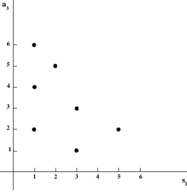
Example 4.4.2. Let S = {s1}, A = {a1,a2,a3} (L = 3) and T = {t1} such that
S < A < T and a3 < a2 < a1. Let us consider J = I(Z) ⊂ C[s1,a3,a2,a1,t1] with
Z = {(1,2,1,0,0),(1,2,2,0,0), (1,4,0,0,0), (1,6,0,0,0), (2,5,0,0,0), (3,1,0,0,0),
(3,3,0,0,0), (5,2,0,0,0)}.Then:
V(JS) ={1,2,3,5}
V(JS,a3) ={(1,2),(1,4),(1,6),(2,5),(3,1),(3,3),(5,2)}
V(JS,a3,a2) ={(1,2,1),(1,2,2)(1,4,0),(1,6,0),(2,5,0),(3,1,0),(3,3,0),(5,2,0)}
Let us consider the projection π :V(JS,a3)→ V(JS). Then:
|π−1({5})|= 1, |π−1({2})|= 1, |π−1({3})|= 2, |π−1({1})|= 3,
so P3
1 = {2,5},
P3
2 = {3},
P3
3 = {1} and
P3
i = ∅, i > 3. This means that
λ(L) = λ(3) = 3 and P3
l is not empty, for l = 1,2,3. Thus the conditions of
Denition 4.4.1 are satised for h=L= 3 (see Fig. 4.1). In the same way, it is easy to verify said conditions also for h = 1,2, and hence the ideal J is stratied with
respect to the A variables.
1 2
2
3 3
4 4
5 5
6 6
s a3
1 1
Figure 4.1: A variety in a stratied case
With the above notation, an immediate consequence of Theorem 3.6 in [GS06] (Theorem 32 in [GS09]) is the following proposition.
Proposition 4.4.3. Let < be any lexicographic term order with S < A < T and aL <aL−1 <· · ·< a1. Let J be a stratied ideal with respect to the A variables. Let
G= GB(J). Then G contains one and only one polynomial g such that: g ∈K[S,aL], T(g) =aLL.
4.4.2 Root multiplicities and Hasse derivative Denition 4.4.4. Let g = P
iaix
i