Quantitative identification of crop disease and nitrogen-water stress in
winter wheat using continuous wavelet analysis
Wenjiang Huang
1,2,4*,
Junjing Lu
3,
Huichun Ye
1,2,4,
Weiping Kong
1,2,
A. Hugh Mortimer
5,
Yue Shi
1,2(1. State Key Laboratory of Remote Sensing Science, Institute of Remote Sensing and Digital Earth, Chinese Academy of Sciences, Beijing 100094, China; 2. Key Laboratory of Digital Earth Science, Institute of Remote Sensing and Digital Earth, Chinese Academy of Sciences,
Beijing 100094, China; 3. Institute of Geographical Science, Hebei Academy of Sciences, Shijiazhuang 050021, China; 4. Hainan Provincial Key Laboratory of Earth Observation, Sanya 572029, Hainan, China;
5. Rutherford Appleton Laboratory, Harwell Science and Innovations Campus, Oxfordshire OX11 0QX, UK)
Abstract: It is necessary to quantitatively identify different diseases and nitrogen-water stress for the guidance in spraying specific fungicides and fertilizer applications. The winter wheat diseases, in combination with nitrogen-water stress, are therefore common causes of yield loss in winter wheat in China. Powdery mildew (Blumeria graminis) and stripe rust (Puccinia striiformis f. sp. Tritici) are two of the most prevalent winter wheat diseases in China. This study investigated the potential of continuous wavelet analysis to identify the powdery mildew, stripe rust and nitrogen-water stress using canopy hyperspectral data. The spectral normalization process was applied prior to the analysis. Independent t-tests were used to determine the sensitivity of the spectral bands and vegetation index. In order to reduce the number of wavelet regions, correlation analysis and the independent t-test were used in conjunction to select the features of greatest importance. Based on the selected spectral bands, vegetation indices and wavelet features, the discriminate models were established using Fisher’s linear discrimination analysis (FLDA) and support vector machine (SVM). The results indicated that wavelet features were superior to spectral bands and vegetation indices in classifying different stresses, with overall accuracies of 0.91, 0.72, and 0.72 respectively for powdery mildew, stripe rust and nitrogen-water by using FLDA, and 0.79, 0.67 and 0.65 respectively by using SVM. FLDA was more suitable for differentiating stresses in winter wheat, with respective accuracies of 78.1%, 95.6% and 95.7% for powdery mildew, stripe rust, and nitrogen-water stress. Further analysis was performed whereby the wavelet features were then split into high-scale and low-scale feature subsets for identification. The accuracies of high-scale and low-scale features with an overall accuracy (OA) of 0.61 and 0.73 respectively were lower than those of all wavelet features with an OA of 0.88. The detection of the severity of stripe rust using this method showed an enhanced reliability (R2 =0.828). Keywords: winter wheat, crop disease, powdery mildew, stripe rust, nitrogen-water stress, continuous wavelet analysis, quantitative identification
DOI: 10.25165/j.ijabe.20181102.3467
Citation: Huang W J, Lu J J, Ye H C, Kong W P, Mortimer A H, Shi Y. Quantitative identification of crop disease and nitrogen-water stress in winter wheat using continuous wavelet analysis. Int J Agric & Biol Eng, 2018; 11(2): 145–152.
1 Introduction
Nitrogen and water stress are common in the agricultural management, causing major yield loss in winter wheat. When environmental conditions meet, crop diseases and pests can occur and spread rapidly[1]. They can cause extremely severe reduction
in yield and quality of winter wheat, and then result in a significant threat to food security[2]. Traditional monitoring methods for
wheat stresses mainly rely upon manual plant inspection, which is time-consuming, less efficient, and unable to monitor the severity of diseases dynamically over large areas[3]. Fortunately, with the
Received date: 2017-05-02 Accepted date: 2017-10-14
Biographies: Junjing Lu, MS candidate, research interests: crop pest and disease monitoring, Email: [email protected]; Huichun Ye, PhD, research interests: application of remote sensing in agriculture, Email: [email protected]; Weiping Kong, PhD, research interests: application of quantitative remote sensing in agriculture, Email: [email protected]; A. Hugh Mortimer, PhD, research interests: data processing, Email: [email protected]; Yue Shi, PhD, research interests: crop pest and disease monitoring, Email: shiyue@ radi.ac.cn.
*Corresponding author: Wenjiang Huang, PhD, Professor, research interests: application of quantitative remote sensing in agriculture, State Key Laboratory of Remote Sensing Science, Institute of Remote Sensing and Digital Earth, Chinese Academy of Sciences, Beijing 100094, China. Tel: +86-10-82178169, Fax: +86-10-82178177, Email: [email protected].
ability to acquire spatially continuous information on land surfaces, remote sensing is an effective way to monitor the severity and scope of diseases and pests for crops[4].
Powdery mildew (Blumeria graminis) and stripe rust (Puccinia striiformis f. sp. Tritici) are two recurrent wheat diseases in China. These two diseases often occur simultaneously under specific temperature and humidity conditions and when the transmission vectors are present. This can be observed in the wheat-growing regions in northern and northwestern China[1]. Given the disease
characteristics, the application of appropriate fungicides is critical to control the outbreak; however, the misuse and overuse of pesticides can also fail to control the disease; by contrast, they pose the risk of soil and groundwater contamination as well[5]. To
detect these diseases is of vital importance. It is well known that the disease pathogens can cause the changes of biochemical and biophysical of crops, such as pigment content, leaf water content and canopy structures, as well as the change of crop leaf colors[5-7].
These changes would further result in the changes of canopy spectral responses in the sensitive spectral regions, such as the increase of reflectance in the red band, and the decrease of reflectance in the near-infrared bands[8,9]. Hyperspectral remote
spectral band regression, vegetation index, and the derivative of spectral features and continuum removal features[10-12]. Huang et
al.[13] showed that stripe rust has strong spectral responses at 630-
687 nm, 740-890 nm, and 976-1350 nm. Then he proposed the normalized photochemical reflectance index (NPRI) based on the hyperspectral data to effectively estimate the disease index (DI) of stripe rust at the leaf level, with a R2 of 0.84[9]. Guan et al.[14]
identified powdery mildew, stripe rust, and nitrogen-water stress by using integrative indices derived from hyperspectral data, they were consist of the Normalized Difference Vegetation Index and Physiological Reflectance Index (NDVI-PhRI), Modified Simple Ratio and Physiological Reflectance Index (MSR-PhRI), and Nitrogen Reflectance Index and Red edge Vegetation Stress Index (NRI-RVSI). Yuan et al.[15] attempted to differentiate stripe rust,
powdery mildew, and aphids by spectral features. As shown in the results, the performance of the discrimination model was satisfactory in general, with an overall accuracy with R2 of 0.75.
Huang et al.[16] investigated classification of different stresses using
new optimized spectral indices (NSIs) extracted from the RELIEF-F algorithm. The results showed that the NSIs were able to detect diseases and distinguish stresses with good reliability.
Recently, the wavelet transform has emerged as an effective time-frequency analysis tool and has now been adopted in different fields[17-19]. Wavelet analysis includes discrete wavelet transform
(DWT) and continuous wavelet transform (CWT). In comparison to DWT, CWT can extract subtle information in spectra through analysis at continuous scales and positions[18,20], and the continuum
position makes the output of CWT comparable to the original spectra. Cheng et al.[19] extracted leaf water content using CWT
and compared the results with traditional methods. It was found that CWT was sensitive to small signals at high and low frequencies. Some studies have begun to focus on the application of CWT in agriculture. Huang et al.[8] reported that
chlorophyll-sensitive bands selected using continuous wavelet analysis (CWA) had a stronger capability in extracting aphid information from spectral measurements than those selected using correlation analysis. Zhang et al.[21] found that features extracted
using CWA had a stronger correlation with and better estimation accuracy for powdery mildew at the leaf level, when compared with conventional spectral features.
The above studies show that CWA can be used to analyze hyperspectral data to distinguish aphids from other diseases and pests. However, there is little attention in the distinction of different diseases and abiotic stress in winter wheat. In this study, we aimed to identify powdery mildew (PM), stripe rust (YR) and nitrogen-water stress (NW) of winter wheat at the canopy scale by the method of CWA, and to compare the performance of continuous wavelet features (WFs) derived from CWA to spectral bands (SBs) and vegetation indexes (VIs). Furthermore, we established the estimation model of DI for the PM and YR diseases.
2 Materials and methods
2.1 Data acquisition
2.1.1 Experiment design and disease index assessment
The study site is located at Xiaotangshan Precision Agriculture Experimental Base, Beijing, China (40.18°N, 116.44°E). There are three experiments in the study, and the filed campaigns were carried out at the filling stage of winter wheat in different years. Experiment 1 for monitoring the infection of PM was conducted in 21st May 2012, 36 plots (4 healthy and 32 diseased plots) were
selected for the investigation and canopy spectral reflectance
measurements. Experiment 2 for monitoring the infection of stripe rust was conducted in 23rd May 2003, 51 plots (5 healthy and
46 disease plots) were selected. Besides, Experiment 3 was the nitrogen-water experiment, conducted in 24th May 2002 and coupled different nitrogen and water treatments. There were four nitrogen treatments (0, 150 kg/hm2, 300 kg/hm2 and 450 kg/hm2)
and four water treatments (0, 225 m3/hm2, 450 m3/hm2, and
675 m3/hm2). According to the recommendation, the control field
was applied with 300 kg/hm2 of nitrogen and 450 m3/hm2 of water.
48 plots (3 healthy and 45 stressed plots) were selected for sampling and canopy spectral reflectance measurements.
Winter wheat was inoculated with powdery mildew and yellow rust in early April by spore inoculation. When investigated, the disease severity was inspected using the five-point method, i.e., in each plot, we selected five symmetric points with an area of about 1 m2, and then 20 wheat samples were randomly investigated in
each selected point and recorded the severity level of each leaf. The severity levels were classified into 9 grades: 0% (i=1), 1% (i=2), 10% (i=3), 20% (i=4), 30% (i=5), 45% (i=6), 60% (i=7), 80% (i=8) and 100% (i=9), in which 0% indicates no incidence of powdery mildew or yellow rust, whereas 100% indicates the highest incidence[12]. The DI was calculated using Equation (1):
( )
i n
DI
k n
× =
×
∑
∑
(1)where, iis the severity level; n is the total number of leaves at each severity level; k is the highest severity level of 9. The DIs of five points within a plot are averaged to represent the disease severity of the plot.
2.1.2 Canopy spectral measurement
Canopy spectra were measured using an ASD FieldSpec Pro FR 2500 (ASD Inc., Boulder, Colorado, USA) under clear sky conditions between 10:00-14:00 (Beijing local time). Spectral data was collected from 350-2500 nm at a spectral resolution of 3 nm for the band 350-1050 nm and 10 nm for the band 1050- 2500 nm. All canopy spectral measurements were taken from a height of 1.3 m above the ground (the height of wheat is 90±3 cm at maturity). The ASD spectrometer was fitted with a 25° field of view probe. A calibration panel was used in the process of measurement, and the spectrum of each investigation point was recorded as an average of 20 scans.
2.2 Methods of data processing and modelling 2.2.1 Spectral normalization
As the spectral reflectance acquired in different years were influenced by the soil and illumination background, spectral normalization was necessary before performing the spectral analysis, because it can reduce the influence of the above differences, but not alter the inherent differences of stressed and healthy samples[22]. The spectral data collected in 2003 and 2012
were taken as an example to illustrate the process of spectral normalization.
Firstly, the average spectrum of healthy wheat samples collected in 2003 was chosen as the baseline measurement. The spectral ratio was calculated by the ratio of the baseline spectral reflectance to the average spectral reflectance of healthy wheat samples collected in the other two years. It is formulated as:
( 03)
( 12)
H i
i
H i Ref Ratio
Ref
= (2)
( 12)H i
Ref are the average spectral reflectance of healthy wheat samples at band i collected in 2003 and 2012, respectively.
Secondly, the spectral normalization in 2012 was calculated as Equation (3).
( 12)H i ( 12)H i i Ref ′ =Ref ×Ratio
(3)
where, Ref( 12)H i′ and Ref( 12)H i are the normalized and original spectral reflectance at band i in 2012; And the spectral reflectance collected in 2002 was normalized in the similar process.
2.2.2 Vegetation indexes
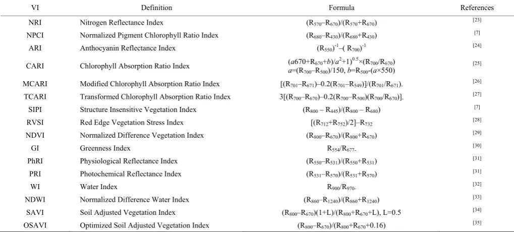
Sixteen VIs (Table 1) were selected to identify PM, YR and
NW stress. The chlorophyll absorption ratio index (CARI), modified chlorophyll absorption ratio index (MCARI) and transformed chlorophyll absorption ratio index (TCARI) are closely related to chlorophyll content. The normalized difference water index (NDWI) and the water index (WI) are associated with water content. The normalized difference vegetation index (NDVI) is sensitive to canopy structure, and soil adjusted vegetation index (SAVI) along with the optimized soil adjusted vegetation index (OSAVI) further reduces the sensitivity of NDVI to the soil background. The physiological reflectance index (PhRI) and photochemical reflectance index are useful to estimate the solar utilization efficiency during development.
Table 1 Summary of vegetation indexes used to identify PM, YR and NW stress
VI Definition Formula References
NRI Nitrogen Reflectance Index (R570–R670)/(R570+R670) [23]
NPCI Normalized Pigment Chlorophyll Ratio Index (R680–R430)/(R680+R430) [7]
ARI Anthocyanin Reflectance Index (R550)-1–( R700)-1 [24]
CARI Chlorophyll Absorption Ratio Index (a670+R670+b)/a2+1)0.5×(R700/R670)
a=(R700–R500)/150, b=R500-(a×550)
[25]
MCARI Modified Chlorophyll Absorption Ratio Index [(R701–R671)–0.2(R701–R549)]/(R701/R671)- [26]
TCARI Transformed Chlorophyll Absorption Ratio Index 3[(R700–R670)–0.2(R700–R500)(R700/R670)]- [27]
SIPI Structure Insensitive Vegetation Index (R800 – R445)/(R800 – R680) [7]
RVSI Red Edge Vegetation Stress Index [(R712+R752)/2]–R732 [28]
NDVI Normalized Difference Vegetation Index (R800–R670)/(R800+R670) [29]
GI Greenness Index R554/R677- [30]
PhRI Physiological Reflectance Index (R550–R531)/(R550+R531) [31]
PRI Photochemical Reflectance Index (R531–R570)/(R531+R570) [31]
WI Water Index R900/R970- [32]
NDWI Normalized Difference Water Index (R860–R1240)/(R860+R1240) [33]
SAVI Soil Adjusted Vegetation Index (R800–R670)(1+L)/(R800+R670+L), L=0.5 [34]
OSAVI Optimized Soil Adjusted Vegetation Index (R800–R670)/(R800+R670+0.16) [35]
2.2.3 Continuous wavelet transform
Compared to the Fourier transform, continuous wavelet transform (CWT) provides the localized frequency and time domains at the same time. The wavelet transform refines each original spectrum at continuum positions and scales according to a wavelet function Ψ(λ). The Mexican Hat wavelet, similar to the shape of the absorption features, was used as the mother wavelet’s basis[17]. Then, the original spectrum can be converted to a series
of continuous wavelet powers that can extract subtle information on disease spectra[36]:
,
( , ) ( ) ( )
f a b
W a b f d
+∞
−∞
=
∫
λ ψ
λ λ
(4),
1 ( )
a b
b a a
−
⎛ ⎞
= ⎜ ⎟
⎝ ⎠
λ
ψ
λ
ψ
(5)where,
ψ λ
( ) is the mother wavelet, f(λ) (λ= 1, 2,…, k, where k is the number of wave bands) is the reflectance spectrum; a is the scaling factor representing the width of the wavelet, and b is the shifting factor representing the position.The CWT converted 1-D reflectance to a 2-D wavelet power scalogram visualized as dimensions of wavelength and scale. For convenient calculation and to not affect the accuracy of CWA, the wavelet coefficients were applied in this study[19,20]. These
wavelet coefficients were decomposed at scales of 2n (n=1, 2,…,
10).
2.2.4 Feature selection of disease discrimination
In order to eliminate the redundancy of spectral bands,
vegetation indexes, and wavelet features, a feature screening process is necessary to identify the most significant features used to discriminate different stresses. Step 1: An independent t-test was conducted to obtain the spectral bands and vegetation indexes that were discrepant between PM & YR, YR & NW, and NW & PM. Step 2: Since wavelet features have strong redundancy with only an independent t-test, both correlation analysis and an independent t-test were used to search correlated (Figures 1a-1c) and discrepant features (Figures 1d-1f). Step 3: The p-values of the correlation analysis and independent t-test indicated the significance of correlation and difference between stressors. Then the intersections were used to screen significant SBs/VIs (p<0.05). For WFs, the overlapping features (p<0.01) had both strong correlation and significant discrepancy under different stresses (Figure 1g).
2.2.5 Stresses discrimination models
To assess and compare the efficiency of SBs, VIs and WFs in stress identification, both algorithms of Fisher’s Linear Discriminate Analysis (FLDA) and a support vector machine (SVM) were applied separately. FLDA aims to find an appropriate projection direction using the covariance matrix to achieve the maximum degree of distinction between each category[37-39]. Meanwhile, SVM was one of methods of machine
learning based on the statistical theory, and it is better than statistical method in solving nonlinear problems[40]. In this study,
Figure 1 Visualization of p-value scalograms of independent t-test and correlation analysis by continuous wavelet analysis
SBs, VIs and WFs were used to discriminate PM, YR, and NW in algorithms of FLDA and SVM. Wheat samples were randomly divided into two datasets: 60% of the samples as the training dataset and the remaining 40% of the samples as the validation dataset. Four indicators were calculated in a confusion matrix to evaluate the accuracy of the models: the overall accuracy (OA), user’s accuracy (U′.sa(%)), producer’s accuracy (P′.sa(%)), and kappa
coefficient.
2.2.6 Estimation model of disease index and validation
Crop disease monitoring can be implemented by identifying different stresses and estimating the DI. Based on the result of stresses discrimination using SBs, VIs and WFs, the best one among the above three spectral features was selected, and then was used to estimate the DI of winter wheat. Considering possible multi-correlation among variables, partial least squares regression (PLSR) was utilized to establish the estimation model of DI. Leave-one-out cross validation approach was used for model validation.
3 Results
3.1 Normalization of original spectral reflectance
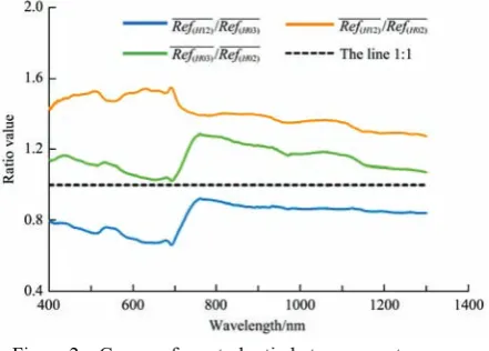
The curves of spectral ratio between any two years (i.e. 2012 vs. 2003, 2012 vs. 2002, and 2003 vs. 2002) are shown in Figure 2. When a band ratio was closer to 1, the differences of data in two different years were smaller. The curves of Ref(H12) Ref(H03)
and Ref(H03) Ref(H02) were closer to 1 than that of
(H12) (H02)
Ref Ref , which implied that the backgrounds of PM and NW were similar to that of YR, whereas the differences of backgrounds between powdery mildew and nitrogen-water were relatively large. Therefore, the average spectrum of healthy samples in 2003 was chosen as the baseline measurement. Then the spectral reflectance of the PM, YR, and NW acquired in different years can be normalized according to Equation (3).
However, the ratio had a certain deviation from 1, perhaps because the data were obtained in different years with different environmental conditions. This also highlighted the necessity of spectral normalization.
Figure 2 Curves of spectral ratio between any two years (i.e. 2012 vs. 2003, 2012 vs. 2002, and 2003 vs. 2002) 3.2 Identification of discrepancies in spectral bands and vegetation indexes
The spectral bands that were significantly screened are shown in Figure 3. It was found that most of the response bands were located in the visible region, and the two spectral ranges at 615-621 nm and 693-696 nm were the most effective to identify PM, YR and NW. This result was consistent with the finding of Graeff et al.[41]. As shown in Table 2, six vegetation indexes were selected,
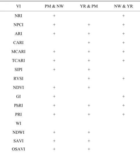
including NPCI, ARI, MCARI, TCARI, PhRI and PRI. NPCI, ARI, PhRI and PRI were more sensitive to the YR during the whole growth stages of winter wheat. Huang et al. reported that the ARI and PRI achieved good performances in the monitoring of crop disease[12], and this was further confirmed by Devadas et al.[7]
indexes, i.e. MCARI and TCARI, can effectively capture the changes of leaf chlorophyll content due to crop diseases and nitrogen-water stress.
Figure 3 Overlapping spectral band selection (the black regions are the selected sensitive bands)
Table 2 Selection of vegetation indexes to identify PM, YR and NW
VI PM & NW YR & PM NW & YR
NRI + + NPCI + + +
ARI + + + CARI + + MCARI + + +
TCARI + + + SIPI + + RVSI + + NDVI + +
GI + + PhRI + + +
PRI + + + WI NDWI + +
SAVI + + OSAVI + +
Note: “+” indicates the selected VIs at a significant level of p-value<0.05.
3.3 Extraction of sensitive and discrepant wavelet features As shown in Figure 1g, the wavelet features screened by overlapping processes formed a number of scatter regions on p-value scalograms. Since features in each region were from sequential positions and scale and they carried the information on superfluous wavelet, the feature with the strongest correlation and most significant difference within each region was determined to represent the spectral information of the feature region (Table 3).
All selected wavelet features were observed in visible, red-edge and near infrared regions. The analysis of the WFs shows that they were mainly distributed in low scales (21-24), whereas the remaining
five WF, i.e. WF1 525 nm, WF3 573 nm, WF4 615 nm, WF7 719 nm, and WF10 809 nm, were in high scales (25-26). They appeared
on green peak, red valley and high reflection platforms in the spectral region, and captured the variations in amplitude of leaf reflectance over a broad spectral interval. The positions of WFs in low scales had a wide distribution, in which WF12 and WF13 embodied the changes in internal plant structure. From their distribution, most of the wavelet features were in the strong absorbed position of chlorophyll in visible regions. WF8, WF9, and WF10 were located at the red edge, the shift of which indicates
a growing condition in crops[42]. WF11, WF12, and WF13
representing plant structure were distributed in the near-infrared shoulder, which is not detected in discrepant spectral bands and vegetation indexes. This was consistent with the result of Cheng et al.[19] who reported that the decomposition of reflectance spectra
with CWT effectively decreased the influence of leaf structural variation. WF13 was related to the water absorption located at 1204 nm, which may suggest significant water stress[20]. Others
were mainly in the green peak and red valley. WF5 and WF6 were distributed in the absorption peaks of chlorophyll b and chlorophyll a. WF7 was weakly related to water absorption. The changes of biochemical and biophysical of crops, such as pigment content, leaf water content and canopy structures would occur after suffering from stresses[5-7]. From these results, all changes of winter wheat
under stresses could be sensitively captured by the wavelet features. Table 3 Locations and scales of stress-sensitive wavelet
features
Wavelet feature Scale Wavelengths/nm p-value
WF1 25 525 0.01
WF2 22 548 0.01
WF3 26 573 0.01
WF4 25 615 0.01
WF5 24 652 0.01
WF6 24 669 0.01
WF7 25 719 0.01
WF8 23 758 0.01
WF9 24 778 0.01
WF10 25 809 0.01
WF11 24 839 0.01
WF12 21 958 0.01
WF13 22 1204 0.01
3.4 Comparison of the performances spectral bands, vegetation indexes and wavelet features in identifying stresses
Table 4 Confusion matrix and classification accuracy
FLDA SVM
PM YR NW sum OA Kappa PM YR NW sum OA Kappa
SBs
PM 24 1 7 32 75.0 0.72 0.58 9 2 21 32 28.1 0.67 0.50
YR 9 37 0 46 80.4 2 37 7 46 80.4
NW 17 1 27 45 60.0 7 1 37 45 82.2
sum 50 39 34 123 18 40 65 123
48.0 94.9 79.4 50.0 92.5 56.9
VIs
PM 20 1 11 32 62.5 0.72 0.59 20 0 12 32 62.5 0.65 0.48
YR 9 37 0 46 80.4 10 33 3 46 71.7
NW 13 0 32 45 71.1 17 1 27 45 60.0
sum 42 38 43 123 47 34 42 123
47.6 97.4 74.4 42.6 97.1 64.3
WFs
PM 25 0 7 32 78.1 0.91 0.86 18 0 14 32 56.3 0.79 0.68
YR 1 44 1 46 95.7 2 41 3 46 89.1
NW 2 0 43 45 95.7 7 0 38 45 84.4
sum 28 44 51 123 27 41 55 123
89.3 100 84.3 66.7 100 69.1
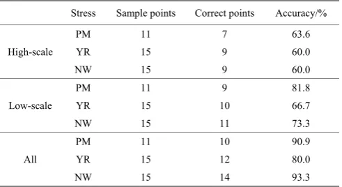
3.5 Information content of high-scale, low-scale, and all WFs. It is obvious that wavelet features were more suitable to discriminate wheat stresses. To analyze further, wavelet features were then split into low-scale (21-24) and high-scale (25-26) feature
subsets. The high-scale, low-scale and all-wavelet features were used as input to detect their informative contribution to stress identification (Table 5). For PM, YR and NW, the recognition accuracies of 63.6%, 60.0% and 60.0% in high-scale features were lower than those in the low scale, which showed accuracies of 81.82%, 66.67% and 73.33%. Nevertheless, the accuracy was best when all wavelet features were used, with values of 90.9%, 80.0%, and 93.3%. The classified result is shown in Figure 4 through group distribution in FLDA according to the canonical discriminant function. Figures 4a-4c are group distributions of high-scale, low-scale, and all-wavelet features, respectively).
Table 5 Identification accuracy for different stresses by wavelet feature subsets
Stress Sample points Correct points Accuracy/%
High-scale
PM 11 7 63.6
YR 15 9 60.0
NW 15 9 60.0
Low-scale
PM 11 9 81.8
YR 15 10 66.7
NW 15 11 73.3
All
PM 11 10 90.9
YR 15 12 80.0
NW 15 14 93.3
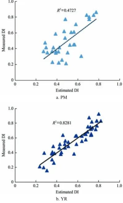
3.6 Estimation of disease index of winter wheat
To further test application capacity of the sensitive WFs, the severity of PM and YR was estimated with PLSR. As shown in Figure 5, both inversion results achieved satisfactory retrieval accuracy with RMSE less than 15%. Moreover, the accuracy of YR had an enhanced level of reliability, with an R2 of 0.828,
suggesting that it is feasible to estimate the severity of winter wheat infected with stripe rust, and this is consistent with the results of Zhang et al.[21] which revealed wavelet features were superior to
traditional spectral features in detecting stripe rust during growth periods.
a. High-scale
b. Low-scale
c. All
a. PM
b. YR
Figure 5 Scatter diagram of estimated DI and WFs-measured disease index
4 Discussion
In this study, the powdery mildew, stripe rust and nitrogen-water stress of winter wheat were quantitatively identified using hyperspectral data. Six VIs, i.e. NPCI, ARI, MCARI, TCARI, PhRI and PRI were retained, their suitability were also demonstrated in the results of Zhang et al.[22], Huang et al.[12] and
Devadas et al.[7]. The selected SBs and spectral bands used in the
VIs were distributed in the visible region, whereas the results showed that the stress or diseases were not completely discriminated in this region. This indicates that the SBs and VIs have the limitation in identifying different stresses. However, unlike the VIs that use mathematical combination of two or three sensitive spectral bands, the analysis of the whole spectral region from the visible to near-infrared bands has proven to be most effective. This is done by looking at the different positions and scales where the CWA shows variation of target information in detail using statistics, and then searching the most sensitive features at multiple scales and positions. In this study, a small number of wavelet features were extracted to form p-value scalograms. The most significant feature in each sequential position was selected, which ensured that it was the most sensitive and discrepant features.
The low-scale components are suitable to capture absorption features of narrow spectral intervals while the high-scale components are well suited to define the overall spectral shape of spectra[18,43,44]. As shown in Table 5, low-scale WFs contributed
more information to identification than high-scale WFs. In this study, narrow absorption features showed changes in pigment, water, and structure caused by different stresses. Because the narrow absorption information and the overall spectral shape were
combined, all WFs were most suitable to differentiate the stresses. Figure 4c distinctly shows that the centroid distance of PM, YR and NW became larger and each category was more concentrated. The CWA is expected to be applied to the hyperspectral imaging spectroscopy data. However, it needs to be validated in the future.
5 Conclusions
Different stresses can influence spectral characteristics in different ways, and it has been shown that continuous wavelet analysis can provide an effective way to identify and discriminate these different stresses. In this study, hyperspectral canopy measurements of PM, YR, and NW were normalized in order to eliminate the effect of background differences. A total of 13 WFs had noticeably superior performance in stress identification with an OA of 0.91 in FLDA, and a producer’s accuracy of YR reaching 100%. Moreover, low-scale WFs contained more information on pigment and water changes, and made the largest contribution to the recognition of stresses. The significant estimation of PM and YR demonstrated the potential application of wavelet features further. In this study, CWA exhibited high practicability in identifying and distinguishing PM, YR and NW. The WFs used to identify stresses were applied directly to estimate the severity, contributing to rapid monitoring of disease occurrence so as to guide the dosage of pesticides. It also has great potential for deriving wavelet features to identify other stresses of crops. However, the CWA method requires hyperspectral data, which increases the cost of monitoring, which in turn limits its use in the field. Moreover, other growth periods (elongation stage, flowering stage) have not been validated in this study. Therefore, the applicability of the method still needs further testing and research.
Acknowledgments
This work was supported by Free Exploration Project of the State Key Laboratory of Remote Sensing Science at Institute of Remote Sensing and Digital Earth, Chinese Academy of Sciences” (17ZY-01), the National Natural Science Foundation of China (61661136004), Hainan Provincial Department of Science and Technology under Grant ( ZDKJ2016021). The authors are grateful to Mr. Weiguo Li, Mrs. Hong Chang, and Zhihong Ma for data collection.
[References]
[1] Li G B, Zeng S M, Li Z Q. Integrated Management of Wheat Pests, 1989. [2] Singh R P, Huerta-Espino J, Roelfs A P. The wheat rusts, 2002.
[3] Bannari A, Khurshid K S, Staenz K, Schwarz J W. A comparison of hyperspectral chlorophyll indices for wheat crop chlorophyll content estimation using laboratory reflectance measurements. IEEE Trans Geosci Remote Sensing, 2007; 45(10): 3063–74.
[4] West J S, Bravo C, Oberti R, Lemaire D, Moshou D, McCartney H A. The potential of optical canopy measurement for targeted control of field crop diseases. Annual Reviews of Phytopathology, 2003; 41: 593–614. [5] Sankaran S, Mishra A, Ehsani R, Davis C. A review of advanced
techniques for detecting plant diseases. Computers and Electronics in Agriculture, 2010; 72(1): 1–13.
[6] Zhang J C, Pu R L, Yuan L, Wang J H, Huang W J, Yang G J. Monitoring powdery mildew of winter wheat by using moderate resolution multi- temporal satellite imagery. PLoS One, 2014; 9(4).
[7] Devadas R, Lamb D W, Simpfendorfer S, Backhouse D. Evaluating ten spectral vegetation indices for identifying rust infection in individual wheat leaves. Precision Agriculture, 2009; 10(6): 459–470.
Powdery Mildew. International Journal of Agriculture and Biology, 2013; 15(1): 34–40.
[9] Huang W J, Liu L Y, Huang M Y, Wang J H. Inversion of the severity of winter wheat yellow rest using proper hyper spectral index. Transactions of the CSAE, 2005; 21(4): 97–103.
[10] Clark R N, Roush T L. Reflectance spectroscopy - quantitative-analysis techniques for remote-sensing applications. Journal of Geophysical Research, 1984; 89(NB7): 6329–6340.
[11] Demetriadesshah T H, Steven M D, Clark J A. High-resolution derivative spectra in remote-sensing. Remote Sensing of Environment, 1990; 33(1): 55–64.
[12] Huang W, Lamb D W, Niu Z, Zhang Y, Liu L, Wang J. Identification of yellow rust in wheat using in-situ spectral reflectance measurements and airborne hyperspectral imaging. Precision Agriculture, 2007; 8(4-5): 187–97.
[13] Huang M Y, Huang W J, Liu L Y, Huang Y D. Spectral reflectance feature of winter wheat single leaf infected with stripe rust and severity level inversion. Transactions of the CSAE, 2004; 20(1): 176–180.
[14] Guan Q S, Huang W J, Jiang J B, Liu L Y. Quantitative identification of stripe rust, powdery mildew and fertilizer-water stress in winter wheat using in-situ hyperspectral data. Sensor Letters, 2014; 12: 1–7.
[15] Yuan L, Huang Y B, Loraamm R W, Nie C W, Wang J H, Zhang J C. Spectral analysis of winter wheat leaves for detection and differentiation of diseases and insects. Field Crops Research, 2014; 156: 199–207. [16] Huang W, Guan Q, Luo J, Zhang J, Zhao J, Liang D, et al. New
optimized spectral indices for identifying and monitoring winter wheat diseases. IEEE Journal of Selected Topics in Applied Earth Observations and Remote Sensing, 2014; 7(6): 2516–24.
[17] Torrence C, Compo GP. A practical guide to wavelet analysis. Bulletin of the American Meteorological Society, 1998; 79(1): 61–78.
[18] Rivard B, Feng J, Gallie A, Sanchez-Azofeifa A. Continuous wavelets for the improved use of spectral libraries and hyperspectral data. Remote Sensing of Environment, 2008; 112(6): 2850–62.
[19] Cheng T, Rivard B, Sanchez-Azofeifa A. Spectroscopic determination of leaf water content using continuous wavelet analysis. Remote Sensing of Environment, 2011; 115(2): 659–670.
[20] Cheng T, Rivard B, Sanchez-Azofeifa G A, Feng J, Calvo-Polanco M. Continuous wavelet analysis for the detection of green attack damage due to mountain pine beetle infestation. Remote Sensing of Environment, 2010; 114(4): 899–910.
[21] Zhang J C, Yuan L, Pu R L, Loraamm R W, Yang G J, Wang J H. Comparison between wavelet spectral features and conventional spectral features in detecting yellow rust for winter wheat. Computers and Electronics in Agriculture, 2014; 100: 79–87.
[22] Zhang J C, Pu R L, Huang W J, Yuan L, Luo J H, Wang J H. Using in-situ hyperspectral data for detecting and discriminating yellow rust disease from nutrient stresses. Field Crops Research, 2012; 134: 165–74. [23] Filella I, Serrano L, Serra J, Penuelas J. Evaluating wheat nitrogen status
with canopy reflectance indexes and discriminant-analysis. Crop Science, 1995; 35(5): 1400–1405.
[24] Gitelson A A, Merzlyak M N, Chivkunova O B. Optical properties and nondestructive estimation of anthocyanin content in plant leaves. Photochemistry and Photobiology, 2001; 74(1): 38–45.
[25] Kim M S, Daughtry C S T, Chappelle E W, McMurtrey J E, Walthall C L. The Use of High Spectral Resolution Bands for Estimating Absorbed Photosynthetically Active Radiation (Apar). Proceedings of the Sixth Symposium on Physical Measurements and Signatures in Remote Sensing, ValD’Isere, France, 1994,17-21; pp.299–306.
[26] Daughtry C S T, Walthall C L, Kim M S, de Colstoun E B, McMurtrey J E. Estimating corn leaf chlorophyll concentration from leaf and canopy
reflectance. Remote Sensing of Environment, 2000; 74(2): 229–239. [27] Haboudane D, Miller J R, Tremblay N, Zarco-Tejada P J, Dextraze L.
Integrated narrow-band vegetation indices for prediction of crop chlorophyll content for application to precision agriculture. Remote Sensing of Environment, 2002; 81(2-3): 416–426.
[28] Merton R, Huntington J. Early simulation of the ARIES-1 satellite sensor for multi-temporal vegetation research derived from AVIRIS. In Summaries of the Eight JPL Airborne Earth Science Workshop, 1999; pp.299–307.
[29] Rouse J W, Haas R H, Scheel J A, Deering D W. Monitoring Vegetation Systems in the Great Plains with ERTS. Proceedings, 3rd Earth Resource Technology Satellite (ERTS) Symposium, 1974, 1; pp.48–62.
[30] Zarco-Tejada P J, Berjon A, Lopez-Lozano R, Miller J R, Martin P, Cachorro V, et al. Assessing vineyard condition with hyperspectral indices: Leaf and canopy reflectance simulation in a row-structured discontinuous canopy. Remote Sensing of Environment, 2005; 99(3): 271–287.
[31] Gamon J A, Penuelas J, Field C B. A narrow-waveband spectral index that tracks diurnal changes in photosynthetic efficiency. Remote Sensing of Environment, 1992; 41(1): 35–44.
[32] Naidu R A, Perry E M, Pierce F J, Mekuria T. The potential of spectral reflectance technique for the detection of Grapevine leafroll-associated virus-3 in two red-berried wine grape cultivars. Computers and Electronics in Agriculture, 2009; 66(1): 38–45.
[33] Gao B C. NDWI - A normalized difference water index for remote sensing of vegetation liquid water from space. Remote Sensing of Environment, 1996; 58(3): 257–66.
[34] Huete A R. A soil-adjusted vegetation index (SAVI). Remote Sensing of Environment, 1988; 25(3): 295–309.
[35] Rondeaux G, Steven M, Baret F. Optimization of soil-adjusted vegetation indices. Remote Sensing of Environment, 1996; 55(2): 95–107.
[36] Bruce L M, Morgan C, Larsen S. Automated detection of subpixel hyperspectral targets with continuous and discrete wavelet transforms. IEEE Trans Geosci Remote Sensing, 2001; 39(10): 2217–2226.
[37] Zhao T, Liang Z Z, Zhang D, Zou Q. Interest filter vs. interest operator: Face recognition using Fisher linear discriminant based on interest filter representation. Pattern Recognition Letters, 2008; 29(13): 1849–1857. [38] Garcia-Allende P B, Conde O M, Mirapeix J, Cobo A, Lopez-Higuera J M.
Quality control of industrial processes by combining a hyperspectral sensor and Fisher's linear discriminant analysis. Sensors and Actuators B-Chemical, 2008; 129(2): 977–84.
[39] Mclachlan G J. Discriminant analysis and statistical pattern recognition Wiley-Interscience, 2004.
[40] Estes W K. Toward a statiscal- the theory of learning (reprinted from phychological review, Vol 57, PG 94, 1950). Psychol Rev, 1994; 101(2): 282–9.
[41] Graeff S, Link J, Claupein W. Identification of powdery mildew (Erysiphe graminis sp tritici) and take-all disease (Gaeumannomyces graminis sp tritici) in wheat (Triticum aestivum L.) by means of leaf reflectance measurements. Central European Journal of Biology, 2006; 1(2): 275–288.
[42] Ahern F J. The effects of bark beetle stress on the foliar spectral reflectance of lodgepole pine. International Journal of Remote Sensing, 1988; 9(9): 1451–1468.
[43] Blackburn G A, Ferwerda J G. Retrieval of chlorophyll concentration from leaf reflectance spectra using wavelet analysis. Remote Sensing of Environment, 2008; 112(4): 1614–1632.
![Compositionnalité et contextes issus de corpus comparables pour la traduction terminologique (Compositionality and Context for Bilingual Lexicon Extraction from Comparable Corpora) [in French]](data:image/gif;base64,R0lGODlhAQABAIAAAP///wAAACH5BAEAAAAALAAAAAABAAEAAAICRAEAOw==)