Modeling streamflow and sediment using SWAT in
Ethiopian Highlands
Hailu Kendie Addis
1,2*, Stefan Strohmeier
3, Feras Ziadat
4,
Nigus Demelash Melaku
1,2, Andreas Klik
1(1. Institute of Hydraulics and Rural Water Management, University of Natural Resources and Life Sciences, Vienna 1190, Austria; 2. Gondar Agricultural Research Center, Gondar, Ethiopia; 3. International Center for Agricultural Research in the Dry Areas,
Amman11110-17198 , Jordan; 4. Food and Agricultural Organization of the United Nations, Rome 00100, Italy)
Abstract: The coincidence of intensive rainfall events at the beginning of the rainy season and unprotected soil conditions after extreme dry spells expose the Ethiopian Highlands to severe soil erosion. Soil and water conservation measures (SWC) have been applied to counteract land degradation in the endangered areas, but SWC efficiency may vary related to the heterogeneity of the landscape. The Soil and Water Assessment Tool (SWAT) model was used to model hydrology and sediment dynamics of a 53.7 km2 watershed, located in the Lake Tana basin, Ethiopia. Spatially distributed stone bund impacts were applied in
the model through modification of the surface runoff ratio and adjustment of a support practice factor simulating the trapped amounts of water and sediment at the SWC structure and watershed level. The resulting Nash-Sutcliffe efficiency (NSE) for daily streamflow simulation was 0.56 for the calibration and 0.48 for the validation period, suggesting satisfactory model performance. In contrast, the daily sediment simulation resulted in unsatisfactory model performance, with the NSE value of 0.07 for the calibration and –1.76 for the validation period and this could be as a result of high intensity and short duration rainfall events in the watershed. Meanwhile, insufficient sediment yield prediction may result to some extent from daily based data processing, whereas the driving runoff events and thus sediment loads occur on sub-daily time scales, probably linked with abrupt gully breaks and development. The calibrated model indicated 21.08 Mg/hm2 average annual sediment yield, which is
far beyond potential soil regeneration rate. Despite the given limits of model calibration, SWAT may support the scaling up and out of experimentally proven SWC interventions to encourage sustainable agriculture in the Ethiopian Highlands. Keywords: SWAT, streamflow, sediment dynamics, soil erosion, soil and water conservation, watershed hydrology DOI: 10.3965/j.ijabe.20160905.2483
Citation: Addis H K, Strohmeier S, Ziadat F, Melaku N D, Klik A. Modeling streamflow and sediment using SWAT in the Ethiopian Highlands. Int J Agric & Biol Eng, 2016; 9(5): 51-66.
1 Introduction
The rise of the human civilizations is directly linked
Received date: 2016-03-19 Accepted date: 2016-09-04 Biographies: Stefan Strohmeier, PhD, research interests: soil and water conservation, Email: [email protected]; Feras Ziadat, PhD, research interests: soil science, Email: [email protected]; Nigus Demelash Melaku, PhD candidate, research interests: soil fertility, Email: [email protected]; Andreas Klik, PhD, Professor, research interests: soil and water conservation, Email: [email protected].
*Corresponding author: Hailu Kendie Addis, PhD candidate, research interests: soil and water conservation. Mailing address: Gondar Agricultural Rresearch Center; P.O. Box 1337, Gondar, Ethiopia; Tel: +251-918711082, Email: [email protected].
with the cultivation of the land and thus, inevitably, with
land degradation[1]. Human interventions, such as
deforestation for agricultural food production, the cultivation of marginal lands, overgrazing and the
exploitation of soil fertility accelerate soil erosion[2] and
subsequent soil depletion is accompanied with reduced
crop productivity[3]. Ongoing land degradation
endangers the agricultural productivity in many areas
around the globe[4], and undoubtedly, the Ethiopian
Highlands are among the most affected. Various impacts and consequences of the severe land degradation in the Ethiopian Highlands have been reported by Hurni
alarming consequence of droughts and low crop productivity, initiated governmental rethinking
concerning rural land management[6]. The Ethiopian
government responded with large scale rehabilitation measures and the establishment of various soil and water conservation (SWC) interventions across the country to
counteract the ongoing soil depletion[6,7].
From the beginning of agricultural activities different
SWC techniques have been developed[8] mainly to retain
soil fertility and thus crop productivity. Various SWC techniques and their variable impacts have been intensively discussed in the literatures [7] and [9]. In particular for the Ethiopian Highlands SWC management through stone bunds was found as sound practice for soil
erosion control[10]. Stone bunds are elevated structures
intersecting a hillslope in specific intervals[7], resulting in
decreased surface runoff and sediment yield through slope length reduction and the creation of a small
retention area[11]. However, SWC interventions are
often uniformly applied across landscapes but may only be reasonable for certain field conditions. In fact, field conditions are often highly variable in the Ethiopian
Highlands[12]. Therefore, site specific assessment of the
most influential watershed processes may be crucial for the development of efficient conservation measures.
At present, many models with a broad spectrum of concepts, which were classified as spatially lumped, spatially distributed, empirical, regression, semi-distributed eco-hydrological model and factorial scoring models, are in use for modelling the rainfall-runoff-soil erosion and sediment transport
processes at different scales[13]. The Soil and Water
Assessment Tool (SWAT) is a semi-distributed eco-hydrological model. SWAT is one of the most widely used watershed models, which was developed by the United States Department of Agriculture-Agricultural
Research Service (USDA-ARS)[14] and can be used to
predict agricultural land management impacts on the hydrological regime of a watershed through simulation of variable soil, land use and management conditions over
long periods[14,15]. In Ethiopia, SWAT has been used in
a number of studies to predict streamflow and sediment
yield[16-21] with different outcomes and recommendations
concerning the usability of the semi-distributed eco-hydrological model for remote landscapes. In fact, large areas of the Ethiopian Highlands are still under investigated and therefore proper model input and particularly calibration data (such as streamflow and sediment yield) are scarce, which might impede proper model calibration and validation in many cases. Various
studies[13,22] have shown that advanced erosion models
suffer from the lack of available input data especially for large scale application. Conclusively, there remains extensive need to evaluate semi-distributed eco-hydrological watershed modeling in the Ethiopian Highlands.
The study reported here was performed in the context of a multidisciplinary international research project that is being conducted within the Gumara-Maksegnit watershed which is located in the Lake Tana basin in the Amhara region of Ethiopia. Integrated watershed research is being conducted, including several soil, crop, hydrology and agro-environmental related analyses, to gain a deeper insight into watershed scale hydrology and land degradation issues, evaluate various soil and water conservation interventions and to aim for an improved livelihood of stakeholders living in the watershed. The spatial assessment of surface runoff and sediment yield within Gumara-Maksegnit study site using SWAT is a key component of the overall research project. The model case study was conducted: (1) to assess the applicability of SWAT for simulating the key watershed processes of a remote and mountainous agricultural watershed, and (2) to evaluate the impact of spatially distributed soil and water conservation (SWC) structures on surface runoff and soil erosion. Eventually, the study aims for the establishment of a well-calibrated semi-distributed eco-hydrological model as a tool for evaluating multiple land management practices suitable for reduction of sediment transport, which can be scaled up to assess proper SWC strategies and to counteract ongoing land degradation at a broader scale.
2 Materials and methods
2.1 Description of the study watershed
Amhara region in northwest Ethiopia between 37°33′00″-
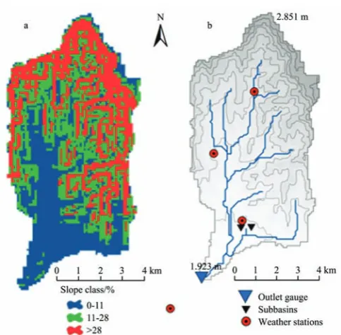
37°37′00″E and 12°24′00″-12°31′00″N (Figure 1).
The confined watershed area is 53.7 km2 based on an
ArcGIS watershed delineation using a 90 m grid Digital Elevation Model (DEM) produced by SRTM
(Shuttle Radar Topography Mission)[23]. The
watershed elevation ranges from 1920 m (outlet) to 2850 m above sea level in the north, while the hillslopes range from nearly flat (<2%) to extremely steep (>70%) (Figure 2a). The northern part of the watershed, Denkez Mountain Ridge, borders to Tekezi Basin, while the Gumara-Maksegnit watershed is part of the Blue Nile River Basin. The watershed geology is dominated
by a Trap Series of Tertiary volcanic eruptions[24],
which are commonly described by their degree of oxidation as exemplified by the frequent dominance of ferric over ferrous iron and by the abundant water
content[24]. The main soils are Cambisol and Leptosol
in the upper and central part of the watershed and Vertisol in the lower part near the outlet. The Gumara-Maksegnit River is the main stream of the study watershed, which part of the Lake Tana drainage basin. Lake Tana is the origin of the Blue Nile River and the largest lake in Ethiopia. The Gumara-Maksegnit River discharges continuously throughout the year and is characterized by several flood events during the rainy season versus drastically decreased flow during the dry season. The climate of the Gumara-Maksegnit watershed is characterized by the ‘Woina Dega’ zone (cool semi-humid) between 1920 m to 2400 m above sea level, and the ‘Dega’ zone (cool) above 2400 m. The majority of the watershed area is located within the cool semi-humid zone at an elevation of 1920 m to 2400 m above sea level. The climate is dominated by distinct wet and dry periods. The wet season typically occurs from June to September and the dry season occurs from November to April, while May and October are transition months. The mean annual rainfall in the watershed is 1200 mm of which more than 90% occurs during the rainy season (June to September). The average monthly maximum and minimum temperatures
recorded from 1997 to 2013 were 31.8°C for March and
10.8°C for January.
Figure 1 Overview of the project watershed area in the northwest Amhara region, Ethiopia
Figure 2 Gumara-Maksegnit watershed maps showing (a) slope classes, and (b) elevation data and location of weather stations and sub-basins included in stone bund experiment assessment discussed
in Section 2.3.5 2.2 SWAT model
The SWAT model is a semi-distributed eco-hydrological continuous event watershed-scale model usable to evaluate the impact of different land management practices on surface and subsurface water movement, sediment, and agricultural chemical yields in complex watersheds with different soil, land-use and management
uses GIS spatial algorithms to spatially link multiple model input data, such as watershed topography (DEM), soil, land use, land management and climatic data. During watershed delineation, the entire watershed is divided into different sub-basins. Then, each sub-basin is discretized into a series of Hydrologic Response Units (HRUs) as the smallest computation unit of a SWAT model, which are characterized by homogeneous soil, land use and slope combinations. Daily climate input data for defined locations (mostly related to ground weather stations) are spatially related to the different sub-basins of the model using a ‘nearest neighbor’ GIS algorithm. Different model outputs, such as surface runoff, sediment yield, soil moisture, nutrient dynamics, crop growth etc., are simulated for each HRU, aggregated and processed to sub-basin level results on a daily time step resolution.
SWAT provides different runoff routing techniques for both surface runoff and streamflow. In this study, surface runoff was computed using the USDA (United States Department of Agriculture) NRCS (Natural
Resources Conservation Service) approach[27], while
channel routing was processed by Muskingum routing
method[28]. The NRCS method was chosen to enable
user friendly and comprehensive consideration of soil and water conservation (SWC) impacts. A number of methods with varying data requirements for evapotranspiration (ET) estimation are incorporated in
SWAT: for this study, the Hargreaves formula[29] was
used. In SWAT, up-land soil erosion is computed based on the Modified Universal Soil Loss Equation
(MUSLE)[29], which allows the consideration of a support
practice factor representing supposed SWC effects on sediment loss.
2.3 Input data
SWAT input data in developing countries (such as Ethiopia) are usually not readily available and are often difficult to collect, and data availability is even more limited for good quality calibration and validation data. Amongst the acquisition of various remote sensing sources for DEM and land use input preparation, comprehensible field sampling and hydrological monitoring were a central task of the Gumara-Maksegnit
watershed study.
2.3.1 DEM (Digital Elevation Model)
For this study, the 90 m grid cell DEM, produced by
SRTM (Shuttle Radar Topography Mission)[23] was used
to obtain the topographic characteristics of Gumara-Maksegnit watershed. Then, the watershed had been divided into three slope steepness classes, namely:
0°-11° (18.77 km2), 11°-28° (17.66 km2) and greater than
28° (17.26 km2) (Figure 2a).
2.3.2 Climate
Climate input data required by SWAT includes daily precipitation, maximum and minimum temperature, relative humidity, half hour rainfall, wind speed and solar radiation. Required daily precipitation and maximum/ minimum air temperature data was collected at four different weather stations located within (three stations) and slightly outside (one station) the watershed (Figure 2b). Daily solar radiation, relative humidity, and wind speed data were recorded at a different metrological
station slightly outside the study watershed (Figure 2b).
The SWAT weather generator[30] was used for simulating
missing daily weather data. The daily climatic data (from January 1, 1997 to December 31, 2013) recorded at the weather station, which was located slightly outside
the watershed (Figure2b) was used to create the monthly
weather statistics using the weather generator. 2.3.3 Land use
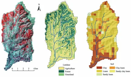
Land cover map for this research was produced on the pixel based supervised classification of 10 m spot satellite image (Figure 3a). The study watershed has three major land-use classes (Figure 3b) and is mainly covered by agricultural land (63.5%) followed by mixed forest (24.3%), and grazing land (12.2%). The agricultural land was further subdivided into six major agricultural
crops: tef (Eragrostis Tef) (30.0%), sorghum (13.2%),
barley (6.9%), fava bean (5.6%), winter wheat (4.3%) and chickpea (3.5%). Tef is a minor cereal crop on a global scale, but a major food grain and lovegrass (lovegrass is commonly used as livestock fodder) in Ethiopia and Eritrea and this annual crop can be grown under a wide
range of conditions[31]. Tef and sorghum are the main
2.3.4 Soil
SWAT requires multiple soil physical and chemical attributes for various soil depths such as soil texture, bulk density, stone content, organic carbon, hydraulic
conductivity, soil erodibility, etc.[32] At least one
software package is available which can be used to calculate the spatial distribution of various soil properties for environmental modeling using selected input
parameters[33]. Nevertheless, good quality field
sampling data may be used preferentially. In this study, an intensive field sampling campaign was carried out to determine various soil properties in a 500 m by 500 m grid over the entire watershed. A total of 234 soil samples were collected using a bucket auger. At each location approximately 2 kg bulk soil samples from different soil layers (0-25 cm), (25-60 cm) and (60-
100 cm) were taken for physical and chemical analysis. Undisturbed soil core cylinder samples were taken from the topsoil layer to determine bulk density following
previously developed procedures[34]. Soil texture was
measured based on an earlier published method[35], and
organic carbon was determined by a wet oxidation
method[36]. Available water content and hydraulic
conductivity for each layer as well as bulk density for the second and third layer were assessed using a
pedo-transfer function developed by Saxton and Rawls[37].
Nevertheless, the most important soil data impacts were manually determined based on the previously described intensive field sampling results. The soil map that describes the distribution of different soil textural classes of the study watershed is presented in Figure 3c.
a. Spot satellite image b. Three major land cover categories c. Soil textural class maps
Figure 3 The Gumara-Maksegnit watershed
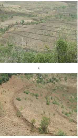
2.3.5 Soil and Water Conservation (SWC) interventions Different SWC practices have been applied in the Gumara-Maksegnit watershed such as stone bunds, micro water harvesting ponds, trenches and semi-circular stone bunds (Figure 4). However, linear (slightly graded) stone bunds are the predominant practice, which affect large agricultural areas in the central and the lower part of the watershed. Locally installed harvesting ponds (four structures applied within the watershed), trenches and semi-circular stone bunds may have a positive effect on
runoff and soil erosion at the field level, but based on their local or minor areal extent, these structures have limited effect on watershed level hydrology or sediment dynamics. Thus, stone bunds were the only SWC interventions considered during watershed modeling and approximately 50% of the study watershed is presently treated with the
stone bunds. As described by Bosshart[11], SWC impacts
effects that occur at each structure. In the course of the Gumara-Maksegnit watershed study, different plot level as
well as sub-basin level experiments were carried out[38] to
investigate the effects of stone bunds on surface runoff and soil loss, and moreover, to enable the implementation of SWC impacted in SWAT modeling. SWAT provides
various options to consider SWC impacts[32] including: (1)
surface runoff may be modified through the adjustment of the runoff ratio (Curve Number) and/or the consideration of a micro-pond (pothole) at the related HRU level, which will also impact soil erosion, and (2) impacts on sediment yield levels via adjustment of the support practice factor (P-factor) and/or the slope length factor (LS) of the
MUSLE[39]. The ideal factors that describe the effect of
stone bunds are the USLE support practice factor (P-factor), the Curve Number and average slope length (SLSUBBSN). In this study, the SLSSUBSN value was modified by editing the HRU (.hru) input table, whereas the P-factor and Curve Number values were modified by editing Management (.mgt) input table.
a
b
Figure 4 Stone bund treated fields (a) and the small channel above the stone bund (b)
The 53.7 km2 Gumara-Maksegnit watershed was
discretized into 15 sub-basins and 2799 HRUs for the SWAT simulations. The highest numbers of HRUs for the study watershed occurred as a result of the 234 user defined soil names, the 3 slope classes as well as the 9
landuse type interactions, however, a coarse DEM mesh used as an input for this study was one of the limitation. The study watershed is composed of a rugged topography with different management practices; thus, the 234 soil sampling points are considered totally different and the study did not set a threshold that eliminates minor soil types. Therefore, every HRU for the study watershed
corresponds with an average area of 1.9 hm2. Similarly,
Zabaleta et al.[40] used 165 HRUs for a 4.8 km2 watershed
in Spain, which averaged about 2.9 hm2 per HRU.
The impact of stone bund SWC structures was simulated through reduction of the Curve Number (CN_2) for surface runoff ratio modification as well as the adjustment of the support practice factor (P-factor) to account for the amount of trapped sediments at the stone bunds. The effect of stone bunds on runoff and soil erosion was initially assessed during the erosion plot experimental campaigns in 2012 and 2013, based on the comparison of treated and untreated sub-basins located in the watershed (this activity is still ongoing). Based on
the plot experiments carried out in 2013[41], stone bund
structures were found to reduce surface runoff by approximately 60% to 80% and sediment yield between 40% to 80%. This is consistent with other plot
experimental findings reported by Adimassu et al.[42],
where stone bunds reduced sediment yield by roughly 50% compared to untreated plots. However, plot experiments tend to reflect optimized stone bund conditions for just a very limited area. In fact, the stone bund plot experiments carried out in Gumara-Maksegnit do not account for cumulative hillslope lengths or the overall length of the stone bund walls and thus how much total area those affect, which may lead to considerably lower SWC impacts at a farm or sub-basin level. For the sub-basin level experiment (Figure 2b), where the
area of each sub-basin is approximately 30 hm2, the
difference of measured surface runoff between treated and untreated sub-basins was around 30%. However, the measured sediment yield declined by only approximately 10% during the 2012 rainy season, which is not consistent with the results reported by
Gebremichael et al.[43] These results include a large
also due to only a few synchronically recorded rainfall events in the treated and untreated sub-basins (Figure 2b). Moreover, the comparability of different sub-basins is limited as a result of the inherent landscape and rainfall related variability, even though the sub-basins border each other and the soil, slope, and land use conditions are generally homogenous. However, the current SWC impact research is ultimately designed to provide comprehensive SWC assessment and conclusive modeling parameters. Hence, as an early stage assessment, the CN_2 was reduced for agricultural HRUs in the treated areas with the target to achieve overall surface runoff reduction of about 30% on treated HRU’s compared to untreated conditions. The P-factor was set equal to 0.85, because: (1) the CN_2 reductions already leads to reduced soil erosion on the treated areas, and (2) as a compromise between plot and sub-basin level sediment yield ratio outcomes. A small range of variability was assigned to the defined CN_2 and P-factor parameter sets during the calibration procedure, which allowed additional minor adjustments during the automated model optimization. These assumptions result in the stone bunds essentially replicating the effects
of terraces[16], in terms of how the average slope length
(SLSUBBSN) is modified to represent terrace effects in cropped landscapes.
2.4 Calibration and validation data
Different calibration approaches can be used in SWAT with respect to frequency and quantity of observation data available for model calibration. Nevertheless, the most powerful calibration is usually achieved through following a specific calibration order as
suggested by Arnold et al.[44] In particular, streamflow
data at the sub-basin or watershed level are required to perform accurate model hydrologic balance and streamflow calibration, followed by calibration of different pollutants such as sediment load, nutrient yields and other water quality variables. The calibration procedure is typically based on initial sensitivity analysis results (using a set of sensitive parameters) and is
executed either manually or automatically[44,45].
Calibrations can be performed manually, which can be
important for clearly understanding some processes[44].
However, automated calibration is more efficient for
some applications[46], especially for complex hydrologic
models. Different datasets may be required to evaluate model performance for different environmental
conditions[45]. However, the number of attributes and
the observation period required for proper consideration of the driving watershed processes may vary from site to site. Long term and good quality data is especially rare for the Ethiopian Highlands. In the present study, the entire simulation period is limited to field observation data from 2011 to 2012 (calibration) and 2013 (validation). The calibration/validation model run was performed with a warm-up period of seven years to minimize the effect of non-equilibrium initial conditions
such as soil moisture or residue cover[47]. In this
research, daily streamflow and sediment yield recorded at the outlet of the watershed were used for both calibration and validation of the model.
Streamflow was obtained by converting quasi-continuous water level (m) records (using pressure transducer) into flow (m/s) based on an experimentally
developed water level and discharge rating curve[48]
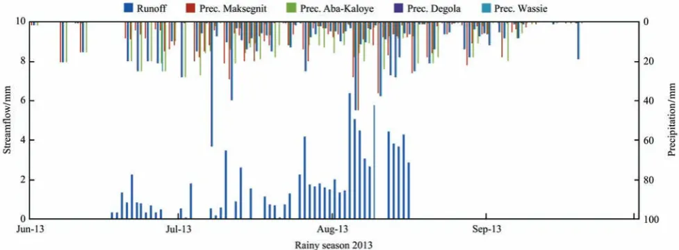
to this, quasi-continuous turbidity readings were controlled and adjusted based on manual bottle sampling throughout the runoff monitoring period. Streamflow and sediment yield, which were derived through multiplying sediment concentration with the according flow volume, were compiled on a daily basis usable for SWAT calibration. Figure 6 shows the derived hydrograph for the main outlet during approximately the four month rainy season in 2013. However, several unmeasured sediment concentration and streamflow data, mainly due to sensor failures or power supply errors,
reveal the challenging monitoring conditions that exist at the site.
Figure 5 Established rating curve at the outlet of Gumara-Maksegnit Watershed[48]
Figure 6 Hydrograph at the main outlet and precipitation data of the four rain gauge stations in Gumara-Maksegnit watershed 2.5 Model efficiency assessment
Efficiency criteria are defined as a mathematical measure of how well a model simulation matches
corresponding observed data[45]. SWAT calibration
procedures, including the SWAT-CUP calibration tool, provide multiple model efficiency criteria to be used as an objective function for model calibration and
validation[49]. The ‘Sequential Uncertainty Fitting 2’
(SUFI-2) procedure, available within SWAT-CUP software, was used to perform model sensitivity analysis,
calibration and validation procedures[49] through iterative
variation of user defined parameter sets. The SUFI-2 algorithm accounts for various sources of uncertainty such as input data uncertainty, conceptual model
uncertainty and parameter uncertainty[50]. In the present
study, the goodness of the modelfit related to streamflow
and sediment yield was assessed based on root mean squared error (RMSE), Nash–Sutcliffe efficiency (NSE), percent bias (PBIAS) and coefficient of determination
(R2). However, during the SWAT-CUP calibration
multiple simulations are executed accounting for the user-adjusted set of parameters and related parameter ranges. This procedure can result in a very large set of simulations, depending on the number of parameters selected for calibration, the user-adjusted range for parameter variation and the selected calibration methodology (including the number of iterations, parameter range discretization etc.).
2.5.1 Root mean square error (RMSE)
The root mean square error (RMSE) has been used as a standard statistical metric to measure model prediction error in meteorology, air quality, and climate research studies; a smaller RMSE value indicates better model
performance[51]. Although RMSE is sensitive to outliers
as it places a lot of weight on large errors, it has been
developed to confirm the reliability of models[52]. The
differences comprising them[53]. The RMSE is calculated with the following equation:
1/2 2 1 1 ( ) n i i i
RMSE E O n =
⎡ ⎤
=⎢ − ⎥
⎣
∑
⎦ (1)2.5.2 Nash-Sutcliffe Efficiency (NSE)
The Nash-Sutcliffe efficiency is a normalized statistic that determines the relative magnitude of the residual variance (“noise”) compared with the measured data
variance (“information”)[54]. The Nash-Sutcliffe
efficiency is calculated as:
2 1 2 1 ( ) 1 ( ) n i i i n i i E O NSE O O = = − = − −
∑
∑
(2)The range of E lies between −∞ and 1.0 with E=1
describing a perfect fit. Values between 0-1.0 are generally viewed as acceptable levels of performance, whereas values <0.0 indicate that the mean observed
value is a better predictor than the model[55].
2.5.3 Percent bias (PBIAS)
Percent bias (PBIAS) is defined as the average tendency of the observed data compared with their
simulated counterparts[56]. The negative values of
PBIAS indicate model overestimation bias, and positive values indicate model underestimation bias. The optimal value of PBIAS is 0.0, with low-magnitude
values indicating accurate model simulation[45]. PBIAS
is calculated with the following equation:
1 1
( ) 100
PBISA ( ) n i i i n i i O E O = = ⎡ − × ⎤ ⎢ ⎥ = ⎢ ⎥ ⎣ ⎦
∑
∑
(3)2.5.4 Coefficient of determination (R2)
The coefficient of determination R2 is defined as the
squared value of the coefficient of correlation[57]. It is
calculated as follows:
2 2 1 2 2 1 1 ( )( ) ( ) ( ) n i i i n n i i i i
O O E E R
O O O E
= = = ⎡ − − ⎤ ⎢ ⎥ = ⎢ − − ⎥ ⎢ ⎥ ⎣ ⎦
∑
∑
∑
(4)where, n is the number of observations or samples; Oi are
observed values; Ei are estimated values; Ō is mean of
observed values; Ē is the mean of estimated values; i is
counter for individual observed and predicted values.
The range of R2 lies between 0 and 1, and describes
how much of the observed value is explained by the
predicted value[55]. A value of 1 means the predicted
value is equal to the observed value, where a value of zero means there is no correlation between the predicted and observed values.
3 Results and discussion
In the Ethiopian Highlands, erratic and intensive rainfalls during the rainy season generate several peak runoff events (Figure 6), exposing steep sloped areas to potentially severe soil erosion. In SWAT, rainfall erosive impacts are estimated mainly as a function of the intensity and duration of rainfall events. The hydrograph at the outlet of the study watershed is dominated by the short period peak flows, occurring several times weekly whereas mean base flow was observed between 1-2 m³/s during rainy season of the calibration periods. Intense rainfall events correspond to peak flows on daily time scale which states that rainwater is routed through the watershed in sub-daily time intervals. This refers to the steep sloped and the rugged mountainous watershed as well as the convective rainfall characteristics in the Ethiopian Highlands. At the outlet, peak discharges of about 30 m³/s have been observed during the 2012 rainy season whereas extreme floods are expected to exceed this amount several times. In contrast, the SWAT model derives maximum mean daily discharges of less than 10 m³/s for the whole calibration period of the 2011 rainy season. This may be due to the daily based runoff computation which can’t adequately account for intense storms of short duration. Rainfall records for the Aba-Kaloye weather station (2011-2013); located in the lower central part of the watershed, suggests that more than 50% of the annual maximum daily rainfall occurs within 30 min time periods during intense storms (Table 1).
Table 1 Annual maximum series rainfall in units of millimeters for Aba-Kaloye weather station
Year 15 m* 30 m 1 h 3 h 6 h 12 h 24 h 48 h 72 h**
2011 20.2 38.6 42.6 47.4 54.6 68.2 74.6 94.4 119.2 2012 16.8 29.6 37.2 40.4 42.8 54.6 58.8 69.6 83.6 2013 15.6 27.8 31.4 36.6 40.2 49.6 52.4 64 79.2 Note: Durations in the table range from 15-min (15 m*) to 72 h (72 h**).
relatively short time periods (sub-daily) and distinct peak flows. Based on a simulation of the whole period of available climate input data (1997-2013), the calibrated model estimates 352 mm of average annual surface runoff, whereas recharge to the deep aquifer is approximately 19 mm, and entirely, more than 31% (373 mm) of rainwater balance is used for evapotranspiration. This low amount of ET in the study watershed was found to be attributable to land use/land cover change, mainly from expanding agricultural activities, as it was
described by Alemu et al.[60] Generally, from field
observation more water is drained out of the watershed as a result of the minimum soil conservation coverage, land use change and the steep slope nature of the study
watershed. In contrast, similar study by Yesuf et al.[58]
showed that 48% of the precipitation becoming ET[58],
while, Gebremicaelet al.[59] reported that 53% of the
precipitation becoming ET.
3.1 Model sensitivity analysis
Sensitivity analysis supports the determination of the driving watershed processes and thus the identification of the most sensitive parameters through the assessment of the rate of change of model outputs with respect to defined
changes of model inputs[44]. Fourteen hydrological
(Table 2) and eight sediment-related (Table 3) parameters were selected for the subsequent SWAT calibration on the bases of the sensitivity analysis. In this study, the CN_2 and channel cover factor were found to be the most sensitive parameters with respect streamflow and sediment yield, respectively.
Table 2 List of model parameters sensitive to streamflow and fitted values in order of ranking
Parameter name Description Adjusted or fitted
parameter value Ranking
r__CN2.mgt* Curve number -0.13 1
r__RCHRG_DP.gw** Deep aquifer percolation fraction 0.3 2
r__GWQMN.gw Threshold depth of water in the shallow aquifer required for return flow to occur (mm H2O) -0.13 3
v__ALPHA_BF.gw Base flow alpha factor (days) 0.019 4 r__GW_REVAP.gw Groundwater “revap” coefficient 0.4 5 v__GW_DELAY.gw Groundwater delay time (days) 110 6 v__CH_K2.rte Effective hydraulic conductivity in main channel alluvium (mm/hr) 82.49 7 v__CH_N2.rte Manning’s “n” value for the main channel -0.00783 8 v__ESCO.hru Plant uptake compensation factor 0.63 9 r__SOL_K(1).sol Saturated hydraulic conductivity -0.52 10 r__REVAPMN.gw Threshold depth of water in the shallow aquifer percolation to the deep aquifer to occur (mm H2O) -0.2 11
r__SLSUBBSN.hru Average slope length (m) 0.01 12 v__SURLAG.bsn Surface runoff lag coefficient 0.3 13 r__SOL_AWC(1).sol Soil available water storage capacity 0.28 14
Note: * The qualifier (r__) refers to relative change in the parameter where the value from the SWAT database is multiplied by 1 plus the fitted value), while (v__) means
the existing parameter value from the SWAT database is to be replaced by the fitted value. ** The extension (e.g., .gw) refers to the SWAT input file where the
respective parameter is located.
Table 3 Model parameters sensitive to sediment yield and fitted values in order of ranking
Parameter name Description Fitted parameter value Ranking
v__ CH_COV2.rte* Channel cover factor 0.8 1
v__ CH_COV1.rte Channel erodibility factor 0.15 2 v__ SPCON.bsn** Linear parameter for calculating the maximum amount of sediment that can be re-entrained during
channel sediment routing 0.009 3
v__ PRF.bsn Peak rate adjustment factor for sediment routing in the main channel 1.4 4 v__ HRU_SLP.hru Average slope steepness (m/m) 0.18 5 v__ SPEXP.bsn Exponent parameter for calculating sediment re-entrained in channel sediment routing 1.35 6 r__ USLE_P.mgt USLE equation support practice factor -0.01 7
v__ RSDIN.hru Initial residue cover (kg/ha) 3400 8 Note: * The qualifier (v__) means the existing parameter value from the SWAT database is to be replaced by the fitted value, while (r__) refers to relative change in the
parameter where the value from the SWAT database is multiplied by 1 plus the fitted value). ** The extension (e.g., .bsn) refers to the SWAT file type where the
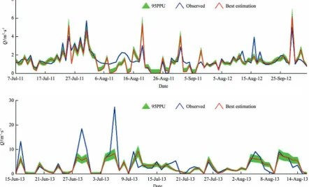
3.2 Model calibration and validation
The automated calibration (SWAT-CUP) for streamflow (Figure 7, top) leads to adequate daily calibration results, and validation (Figure 7, bottom) indicates satisfactory model fit according to the
assessment criteria suggested by Moriasi et al.[45,61] For
the calibration period NSE=0.56, PBIAS=6%, R2=67 and
RMSE=0.62, while for the validation period NSE=0.48,
PBIAS=18%, R2=53 and RMSE=3.4. Meanwhile, the
measured peak flows on the same day often over-predicted for the calibration period and under-
predicted for the validation period (Figure 7). Some of the previously published SWAT studies for smaller watersheds in the northeast and northwest of Ethiopia
tend to show weaker hydrologic results[18,21], which is an
indication that it may be difficult to accurately represent processes and thus obtain better results for smaller watersheds. Nevertheless, obvious correspondence of the hydrographs of observed and simulated streamflow (Figure 7) for both, the calibration and validation period, indicates that SWAT is capable to simulate the hydrological regime of Gumara-Maksegnit watershed.
Figure 7 Observed and simulated daily streamflow hydrograph at the outlet of Gumara-Maksegnit watershed, calibration (top) and validation (bottom)
In contrast, the sediment simulation results were unsatisfactory, especially during the validation period, which is shown by the low or even negative NSE values (i.e. 0.07 for the calibration period and –1.76 for the validation period). The low sediment yield fit is not surprising, particularly in highly erosive regions, where abrupt gully development may affect daily loads
significantly. However, Betrie et al.[16] reported that the
fit between the model daily sediment predictions and the observed concentrations showed good agreement as indicated by very good values of the NSE=0.88 for the calibration period and NSE=0.83 for the validation period at El Diem gauging station. During the calibration of
streamflow about 39% of the data and during the validation period about 31% of the data were bracketed by 95PPU, while during daily sediment yield simulation around 18% of the data were bracketed for the calibration period and 13% of the data were bracketed for the
validation period by 95PPU. The calculated R-factors
of some errors in the data input sources, data preparation
and parameterization[62]. Moreover, the uncertainties
might also be as a result of human and instrumental errors
during data processing[63]. Even though kinematic wave
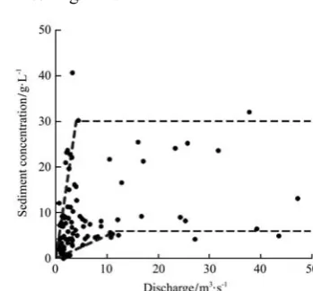
runoff routing is used in the model, peaks of erosional forces of the channel runoff might be underestimated, especially in gully regions of changing flow directions because of gully meanders and/or locally changed flow conditions. Some of the potential reasons for such unsatisfactory sediment yield simulations could probably be, the length of overall measured data, which is quite short, strong hydrological heterogeneity and poor monitoring data as well as the use of USLE (or similar) equations in areas where rainfall happens under the form of short intense rainfall events. Nevertheless, calibration (and validation) of sediment yield on a monthly basis may give much better results, but due to plenty of gaps within the observed data, monthly balancing is not possible for this study. The trends as well as the order of magnitudes of sediment yield seem to be achieved through modeling, and therefore, the model may be able to describe long-term soil erosion characteristics, even if the event based predictions are uncertain. In this study, sediment concentration was also manually sampled at three stages of various flood events. Although selectively sampled sediment data may not be suitable for daily based model calibration, sediment data was used to establish a relation between runoff and sediment concentration (Figure 8). Based on the manual bottle sampling upper and lower boundaries of the expected sediment yield for certain discharge was defined. Though it is commonly accepted that observed
data are inherently uncertain[45], simulated sediment yield
was compared to the expected sediment yield (Figure 9),
and the observed sediment yield ranged from 2.9 Mg/hm2
to 27.6 Mg/hm2, whereas the calibrated model predicted
10.0 Mg/hm2 sediment yield for the observed period and
21.08 Mg/hm2 annually. Similarly, Setegn et al.[19] used
SWAT to simulate the sediment yield simulations for the Anjeni, a small watershed in the northern highlands of Ethiopia, using different slope classifications and the results showed a very high spatial variability for the obtained annual sediment yields, which ranged from 0 to
more than 65 Mg/hm2.
Figure 8 Scatterplot of discharge and sediment concentration of the manual bottle sampling at the main outlet, where dashed lines indicate the lower and upper defined limit of the expected relation
between discharge and sediment concentration
Figure 9 Comparison of the observed range of daily sediment yield (manual bottle sampling) and the simulated daily sediment
yield at the main outlet of the watershed
Although stone bunds reduce the slope length, and decrease overland flow and sheet erosion, the calibrated model still predicted average annual sediment yields which were higher than the potential soil regeneration rate. This indicates a need for expanding SWC practices in the Gumara-Maksegnit watershed to further mitigate soil erosion problems.
Compared to other studies from the literature, Gumara- Maksegnit watershed study may provide conclusive results, for example, SWAT was applied for streamflow simulation of Gedeb catchment, located at the upper Blue
Nile River basin[12], which resulted in unsatisfactory
model performance for both calibration and validation
period. However, Koch[12] pointed out various reasons
for unsatisfactory model results, which seem also valid for the Gumara-Maksegnit case study; i.e., poor monitoring data, strong hydrological heterogeneity and a
difficult and remote terrain. In contrast, Setegn et al.[19]
equal to 0.81 during calibration) for monthly based sediment yield of Anjeni-gauged watershed. This may indicate a well performing model on one hand, but on the other hand the reasonable calibration result also demonstrates typical increasing accuracy of sediment yield prediction for monthly based assessment. Typically, model simulations show a much better fit as
the comparison time scale increases[14,64,65]. There are
also a number of previous SWAT studies in Ethiopia, which documented satisfactory streamflow results including studies that report daily comparisons within the
Lake Tana drainage area[17,20]. However, these are for
larger systems with longer overall observed data versus the smaller Gumara-Maksegnit watershed analyzed in this study with quite short measured data.
Generally, this study documented insufficiencies for matching daily based sediment yield simulation with observed data; this might be a result of poor monitoring data (e.g. short observation period, uncertain data inherent of the measurement technique, occasional data gaps, etc.). Moreover, missing records inhibit the model assessment on a larger time scale (such as monthly or yearly), which typically increases the goodness of the model fit. Hence, especially remote watershed modeling suffers from lack of continuous and good quality data, which has to be considered for semi-distributed eco-hydrological based modeling approaches for such areas.
4 Conclusions
In this research, SWAT watershed modeling was performed to describe the driving hydrological and
sediment transport related processes of a 53.7 km2
watershed in the Ethiopian Highlands. The collected model input data, either from remote earth observation or direct field sampling, are supposed to match SWAT requirements, but limited monitoring data, strong hydrological heterogeneity and poor monitoring data as well as the use of USLE (or similar) equations in areas where rainfall happens under the form of short intense rainfall events are inevitably connected with a large model uncertainty. Another source of uncertainty is the simulated stone bund impacts applied through the surface
runoff ratio (Curve Number) and support practice factor (P-factor) modification. Model calibration executed through the SWAT-CUP software resulted in satisfactory model performance regarding streamflow. However, poor agreement between daily observed and simulated sediment yield resulted as indicated by the NSE=0.07 for the calibration period and –1.76 for the validation period. Nevertheless, overall sediment dynamics and the order of magnitude of various erosion events may be achieved through SWAT simulation. Because of acceptable streamflow simulation (NSE=0.56 for the calibration period and 0.48 for the validation period), but considerable imprecise daily sediment yield prediction at the same time, it is possible that fluctuating sediment processes are influenced by abrupt gully bank breaks and gully network development. Highly variable sediment transport in the main stream may be also a result of distinct sub-daily runoff characteristics of the Gumara-Maksegnit River, and therefore, daily based rainfall and streamflow processing may be limited to describe variable sub-daily peak wave characteristics, inherently linked with variable sediment yield characteristics.
Based on the calibrated SWAT model, the long-term average annual runoff at the main outlet was predicted to be 352 mm, while approximately one third of annual rainfall amount (373 mm) becomes evapotranspiration.
The model predicts 21.08 Mg/hm2 as an average annual
Acknowledgements
The authors thank the Austrian Development Agency (ADA) as well as CGIAR Water Land and Ecosystems (WLE) for providing the financial support. We also thank the Amhara Regional Agricultural Research Institute (ARARI) for constant support and guidance. We thank the students from BOKU University Vienna for their kind assistance and their patient implementation of various field experimental trails. Last but not least, we especially thank the staff from Gondar Agricultural Research Center for their frequent technical and logistical support and also for creating sincere working environment.
[References]
[1] Cerdà A, Flanagan D C, Bissonnais Y L, Boardman J. Soil erosion and agriculture. Soil and Tillage Research, 2009; 106(1): 107–108. doi: 10.1016/j.still.2009.1
[2] Wolka K, Moges A, Yimer F. Effects of level soil bunds and stone bunds on soil properties and its implications for crop production: the case of Bokole watershed, Dawuro zone, Southern Ethiopia. Agricultural Science, 2011; 2(3): 357–363. doi: 10.4236/as.2011.23047
[3] Nyssen J, Poesen J, Mitiku H, Moeyersons J, Deckers J. Tillage erosion on slopes with soil conservation structures in the Ethiopian highlands. Soil and Tillage Research, 2000; 57(3): 115–127. doi: 10.1016/S0167-1987(00)00138-0 [4] Boardman J. Soil erosion science: Reflections on the
limitations of current approaches. Catena, 2006; 68(2): 73–86. doi: 10.1016/j.catena.2006.03.007
[5] Hurni H, Pimentel D. Land degradation, famine, and land resource scenarios in Ethiopia. In: Pimentel D. (Ed.) World soil erosion and conservation. Cambridge University Press, 1993; pp. 27–61.
[6] Hurni H. Degradation and conservation of the resources in the Ethiopian highlands. Mountain Research and Development, 1988; 8(2/3): 123–130. doi: 10.2307/3673438
[7] Herweg K, Ludi E. The performance of selected soil and water conservation measures—case studies from Ethiopia and Eritrea. Catena, 1999; 36(1): 99–114. doi: 10.1016/ S0341-8162(99)00004-1
[8] Morgan R P C. Soil erosion and conservation. Longman Scientific & Technical, J. Wiley, 1995. ISBN: 978-1-4051-4467-4
[9] Teshome A, Rolker D, Graaff J D. Financial viability of soil and water conservation technologies in northwestern
Ethiopian highlands. Applied Geography, 2013; 37(1): 139–149. doi: 10.1016/j.apgeog.2012.11.007
[10] Nyssen J, Poesen J, Desta G, Vancampenhout K, Daes M, Yihdego G, et al. Interdisciplinary on-site evaluation of stone bunds to control soil erosion on cropland in northern Ethiopia. Soil & Tillage Research, 2007; 94(1): 151–163. doi: 10.1016/j.still.2006.07.011
[11] Bosshart U. Catchment Discharge and Suspended Sediment Transport as Indicators of Physical Soil and Water Conservation in the Minchet Catchment, Anjeni Research Unit, Soil Conservation Research Report 40, University of Berne, Berne, Switzerland, 1997.
[12] Koch F J, Van Griensven A, Uhlenbrook S, Tekleab S, Teferi E. The Effects of land use change on hydrological responses in the Choke Mountain Range (Ethiopia)—A new approach addressing land use dynamics in the model SWAT, International Environmental Modeling and Software Society (iEMSs). In Proceedings of 2012 International Congress on Environmental Modeling and Software Managing Resources of a Limited Planet, Sixth Biennial Meeting, Leipzig, Germany, 1–5 July 2012. [13] Vente D J, Poesen J, Verstraeten G, Govers G, Vanmaercke
M, Rompaey A V, et al. Predicting soil erosion and sediment yield at regional scales: Where do we stand? Earth-Science Reviews, 2013; 127(2): 16–29. doi: 10.1016/j.earscirev.2013.08.014
[14] Gassman P W, Reyes M R, Green C H, Arnold J G. The soil and water assessment tool: historical development, applications, and future research directions. Transactions of the ASABE, 2007; 50(4): 1211–1250. doi: 10.13031/ 2013.23637
[15] Gassman P W, Wang Y K. IJABE SWAT Special Issue: Innovative modeling solutions for water resource problems. Int J Agric & Biol Eng, 2015; 8(3): 1–8. doi: 10.3965/ j.ijabe.20150803.1763
[16] Betrie G D, Mohamed Y A, van Griensven A, Srinivasan R. Sediment management modelling in the Blue Nile Basin using SWAT model. Hydrology and Earth System Sciences, 2011; 15(3): 807–818. doi: 10.5194/hess-15-807-2011 [17] Mengistu D T, Sorteberg A. Sensitivity of SWAT
simulated streamflow to climatic changes within the Eastern Nile River basin. Hydrology and Earth System Sciences, 2012; 16(2): 391–407. doi: 10.5194/hess-16-391-2012 [18] Schmidt E, Zemadim B. Expanding sustainable land
management in Ethiopia: Scenarios for improved agricultural water management in the Blue Nile. Agricultural Water Management, 2015; 158: 166–178. doi: 10.1016/j.agwat. 2015.05.001
Modeling of sediment yield from Anjeni-Gauged watershed, Ethiopia using SWAT model. Journal of the American Water Resource Association, 2010; 46(3): 514–526. doi: 10.1111/j.1752-1688.2010.00431.x
[20] Wosenie M D, Verhoest N, Pauwels V, Negatu T A, Poesen J, Adgo E, et al. Analyzing runoff processes through conceptual hydrological modeling in the Upper Blue Nile Basin, Ethiopia. Hydrology and Earth System Sciences, 2014; 18(12): 5149–5167. doi: 10.5194/hessd-11-5287- 2014
[21] Yesuf H M, Assen M, Alamirew T, Melesse A M. Modeling of sediment yield in Maybar gauged watershed using SWAT, northeast Ethiopia. Catena, 2015; 127: 191–205. doi: 10.1016/j.catena.2014.12.032
[22] Rompaey A J V, Govers G. Data quality and model complexity for regional scale soil erosion prediction. International Journal of Geographical Information Science, 2002; 16(7): 663–680. doi: 10.1080/13658810210148561 [23] Jarvis A, Reuter H I, Nelson A, Guevara E. Hole-filled
SRTM for the globe Version 4. Available CGIAR-CSI SRTM 90m Database Httpsrtm Csi Cgiar Org, 2008.
[24] Mohr P A. The geology of Ethiopia. University College of Addis Ababa Press, Ethiopia. 1963.
[25] Arnold J G, Srinivasan R, Muttiah R S, Williams J R. Large area hydrologic modeling and assessment part I: Model development. Journal of the American Water Resources Association, 1998; 34(1): 73–89. doi: 10.1111/j.1752-1688. 1998.tb05961.x
[26] Olivera F, Valenzuela M, Srinivasan R, Choi J, Cho H, Koka S, et al. ARCGIS-SWAT: A geodata model and GIS interface for SWAT. Journal of the American Water Resources Association, 2006; 42(2): 295–309. doi: 10.1111/j.1752-1688.2006.tb03839.x
[27] Baker T J, Miller S N. Using the Soil and Water Assessment Tool (SWAT) to assess land use impact on water resources in an East African watershed. Journal of Hydrology, 2013; 486(8): 100–111. doi: 10.1016/j.jhydrol. 2013.01.041
[28] Neitsch S L, Arnold J G, Kiniry J R, Williams J R. Soil and Water Assessment Tool Theoretical Documentation Version 2009: TR-406. Texas Water Resources Institute, College Station, TX. 2011.
[29] Williams J R, Berndt H D. Sediment yield prediction based on watershed hydrology. Transactions of the ASABE, 1977; 20(6): 1100–1104. doi: 10.13031/2013.35710
[30] Schuol J, Abbaspour K C. Using monthly weather statistics to generate daily data in a SWAT model application to West Africa. Ecological Modelling, 2007; 201(3): 301–311. doi: 10.1016/j.ecolmodel.2006.09.028
[31] Ayele M, Doleže J, Van Duren M, Brunner H, Zapata-Arias F J. Flow cytometric analysis of nuclear genome of the Ethiopian cereal tef [Eragrostis tef (Zucc.) Trotter]. Genetica, 1996; 98(2): 211–215. doi: 10.1007/BF00121369 [32] Neitsch S L, Arnold J G, Kiniry J R, Williams J R. Soil and Water Assessment Tool–Theoretical Documentation, Version 2005. Grassland, Soil and Water Research Laboratory, Agricultural Research Service, Blackland Research Center, Texas Agricultural Experiment Station, Texas. 2005.
[33] Ziadat F M, Dhanesh Y, Shoemate D, Srinivasan R, Narasimhan B, Tech J. Soil-Landscape Estimation and Evaluation Program (SLEEP) to predict spatial distribution of soil attributes for environmental modeling. International Int J Agric & Biol Eng, 2015; 8(3): 158–172. doi: 10.3965/ j.ijabe.20150803.1270
[34] Smith K A, Mullins C E. Soil analysis: physical methods. New York: Marcel Dekker, Inc.. 1991.
[35] Gee G W, Or D. 2.4 Particle-size analysis. In Dane J H, Topp G C (eds). Methods of soil analysis. Part 4. Physical methods. Madison, WI: Soil Sci. Soc. Am. Book Ser. 5. 2002; pp. 255-293.
[36] De Vos B, Lettens S, Muys B, Deckers J A. Walkley–Black analysis of forest soil organic carbon: recovery, limitations and uncertainty. Soil Use and Management, 2007; 23(3): 221–229. doi: 10.1111/j.1475-2743.2007.00084.x
[37] Saxton K E, Rawls W J. Soil water characteristic estimates by texture and organic matter for hydrologic solutions. Soil Science Society of America Journal, 2006; 70(5): 1569–1578. doi: 10.2136/sssaj2005.0117
[38] Brenner C, Strohmeier S, Ziadat F, Klik A. Soil conservation measures in the Ethiopian Highlands: The effectiveness of stone bunds on soil erosion processes. In EGU General Assembly Conference Abstracts, 2013; vol. 15, pp. 5392. Vienna.
[39] Williams J R. Sediment routing for agricultural watersheds. Journal of the American Water Resources Association (JAWRA), 1975; 11(5): 965–974. doi: 10.1111/j.1752- 1688.1975.tb01817.x
[40] Zabaleta A, Meaurio M, Ruiz E, Antigüedad I. Simulation climate change impact on runoff and sediment yield in a small watershed in the Basque Country, northern Spain. Journal of Environmental Quality, 2014; 43: 235–245. doi:10.2134/jeq2012.0209
[41] Rieder J, Strohmeier S, Demelash N, Ziadat F, Klik A. Investigation of the impact of stone bunds on water erosion in northern Ethiopia. In EGU General Assembly Conference Abstracts, 2014; vol. 16, p. 3885. Vienna.
in the central highlands of Ethiopia. Land Degradation & Development, 2012; 25(6): 554–564. doi: 10.1002/ldr.2182 [43] Gebremichael D, Nyssen J, Poesen J, Deckers J, Haile M,
Govers G, et al. Effectiveness of stone bunds in controlling soil erosion on cropland in the Tigray Highlands, northern Ethiopia. Soil Use and Management, 2005; 21(3): 287–297. doi: 10.1111/j.1475-2743.2005.tb00401.x
[44] Arnold J G, Moriasi D N, Gassman P W, Abbaspour K C, White M J, Srinivasan R, et al. SWAT: Model use, calibration, and validation. Transactions of the ASABE, 2012; 55(4): 1491–1508. doi: 10.13031/2013.42256 [45] Moriasi D N, Arnold J G, Van Liew M W, Bingner R L,
Harmel R D, Veith T L. Model evaluation guidelines for systematic quantification of accuracy in watershed simulations. Transactions of the ASABE, 2007; 50(3): 885–900. doi: 10.13031/2013.23153
[46] Balascio C C, Palmeri D J, Gao H. Use of a genetic algorithm and multi-objective programming for calibration of a hydrologic model. Transactions of the ASABE, 1998; 41(3): 615–619. doi: 10.13031/2013.17229
[47] Gitau M W. A quantitative assessment of BMP effectiveness for phosphorus pollution control: The Town Brook Watershed. NY. Pennsylvania State University. 2003.
[48] Zehetbauer I, Strohmeier S, Ziadat F, Klik A. Runoff and sediment monitoring in an agricultural watershed in the Ethiopian Highlands. In EGU General Assembly Conference Abstracts, 2013; vol. 15, p. 5640. Vienna.
[49] Abbaspour K C, Vejdani M, Haghighat S. SWATCUP calibration and uncertainty programs for SWAT. In Proc. Intl. Congress on Modelling and Simulation (MODSIM’07), 2007; 1603-1609. L. Oxley and D. Kulasiri, eds. Melbourne, Australia: Modelling and Simulation Society of Australia and New Zealand.
[50] Gupta H V, Beven K J, Wagener T. Model calibration and uncertainty estimation. In Encyclopedia of Hydrological Sciences, 2006; 11–131.
[51] Chai T, Draxler R R. Root mean square error (RMSE) or mean absolute error (MAE)?–Arguments against avoiding RMSE in the literature. Geoscientific Model Development, 2014; 7(3): 1247–1250. doi: 10.5194/gmd-7-1247-2014 [52] Hernandez-Stefanoni J L, Ponce-Hernandez R. Mapping
the spatial variability of plant diversity in a tropical forest: comparison of spatial interpolation methods. Environmental Monitoring and Assessment, 2006; 117: 307–334. doi: 10.1007/s10661-006-0885-z
[53] Willmott C J. Some comments on the evaluation of model
performance. Bulletin of the American Meteorological Society, 1982; 63(11): 1309–1313.
[54] Nash J E, Sutcliffe J V. River flow forecasting through conceptual models: Part I. A discussion of principles. Journal of Hydrology, 1970; 10(3): 282–290. doi: 10.1016/0022- 1694(70)90255-6.
[55] Krause P, Boyle D P, Bäse F. Comparison of different efficiency criteria for hydrological model assessment. Advances in Geosciences, 2005; 5(5): 89–97.
[56] Gupta H V, Sorooshian S, Yapo P O. Status of automatic calibration for hydrologic models: Comparison with multilevel expert calibration. Journal of Hydrologic Engineering, 1999; 4(2): 135–143.
[57] Stigler S M. Francis Galton’s account of the invention of correlation. Statistical Science, 1989; 4(2): 73–79.
[58] Yesuf H M, Melesse A M, Zeleke G, Alamirew T. Streamflow prediction uncertainty analysis and verification of SWAT model in a tropical watershed. Environmental Earth Sciences, 2016; 75(9): 1–6.
[59] Gebremicael T G, Mohamed Y A, Betrie G D, Zaag P V D, Teferi E. Trend analysis of runoff and sediment fluxes in the Upper Blue Nile basin: A combined analysis of statistical tests, physically-based models and landuse maps. Journal of Hydrology, 2013; 482(2): 57–68. doi: 10.1016/j.jhydrol. 2012.12.023
[60] Alemu H, Kaptué A T, Senay G B, Wimberly M C, Henebry G M. Evapotranspiration in the Nile Basin: Identifying Dynamics and Drivers, 2002–2011. Water, 2015; 7(9): 4914–4931. doi: 10.3390/w7094914
[61] Moriasi D N, Gitau M W, Pai N, Daggupati P. Hydrologic and water quality models: Performance measures and evaluation criteria. Transactions of the ASABE, 2015; 58(6): 1763–1785. doi: 10.13031/trans.58.10715
[62] Freer J, Beven K, Ambroise B. Bayesian estimation of uncertainty in runoff prediction and the value of data: An application of the GLUE approach. Water Resource Research, 1996; 32(7): 2161–2173.
[63] Singh V, Bankar N, Salunkhe S S, Bera A K, Sharma J R. Hydrological stream flow modelling on Tungabhadra catchment: parameterization and uncertainty analysis using SWAT CUP. Current Science, 2013; 104(9): 1187–1199. [64] Engel B, Storm D, White M, Arnold J, Arabi M. A
hydrologic/ water quality model application protocol. Journal of the American Water Resources Association. 2007; 43(5): 1223–1236.