New Connectivity Topological Indices

Vol. 20, No. 1, 2019, 1-8

ISSN: 2279-087X (P), 2279-0888(online) Published on 26 June 2019

www.researchmathsci.org

DOI: http://dx.doi.org/10.22457/apam.622v20n1a1

1

Annals of

New Connectivity Topological Indices

V.R.Kulli

Department of Mathematics

Gulbarga University, Gulbarga 585106, India e-mail: [email protected]

Received 1 June 2019; accepted 25 June 2019

Abstract. New degree based graph indices called Kulli-Basava indices were introduced and studied their mathematical and chemical properties which have good response with mean isomer degeneracy. In this study, we introduce the sum connectivity Kulli-Basava index, product connectivity Kulli-Basava index, atom bond connectivity Kulli-Basava index and geometric-arithmetic Kulli-Basava index of a graph and compute exact formulas for some special graphs.

Keywords: Connectivity Kulli-Basava indices, wheel, gear, helm graphs

AMS Mathematics Subject Classification (2010): 05C05, 05C07, 05C12, 05C35 1. Introduction

Let G be a finite, simple connected graph with vertex set V(G) and edge set E(G). The degree of dG(v) of a vertex v is the number of vertices adjacent to v. The degree of an edge e = uv in G is defined by dG(e) = dG(u) + dG(v) – 2. The open neighborhood NG(v) of a vertex v is the set of all vertices adjacent to v. The edge neighborhood of a vertex v is the set of all edges incident to v and it is denoted by Ne(v). Let Se(v) denote the sum of the degrees of all edges incident to a vertex v. We refer to [1] for undefined term and notation.

A topological index is a numerical parameter mathematically derived from the graph structure. Several topological indices have been considered in Theoretical Chemistry, see [2, 3].

The first and second Kulli-Basava indices were introduced in [4], defined as

( ) ( ) ( )

( )

1 e e ,

uv E G

KB G S u S v

∈

 

=

∑

 + 

( ) ( ) ( )

( )

2 e e .

uv E G

KB G S u S v

∈

=

∑

The first and second hyper Kulli-Basava indices were introduced by Kulli [5], defined as

( ) ( ) ( )

( )

2

1 e e ,

uv E G

HKB G S u S v

∈

 

=

∑

 +  ( ) ( ) ( )

( )

2

2 e e .

uv E G

HKB G S u S v

∈

 

2

We introduce the sum connectivity Kulli-Basava index, product connectivity Kulli-Basava index, atom bond connectivity Kulli-Basava index, geometric-arithmetic Kulli-Basava index and reciprocal Kulli-Basava index of a graph, defined as

( )

( ) ( )

( )

1

,

uv E G

e e

SKB G

S u S v

∈ =

+

∑

( )

( ) ( ) ( )

1 ,

uv E G _{e e}

PKB G

S u S v

∈

=

∑

( ) ( ) ( )

( ) ( ) ( )

2 ,

e e

uv E G e e

S u S v ABCKB G

S u S v

∈

+ −

=

∑

( ) ( ) ( )

( ) ( )

( )

2

,

e e

uv E G e e

S u S v GAKB G

S u S v

∈ =

+

∑

( ) ( ) ( )

( )

.

e e

uv E G

RKB G S u S v

∈

=

∑

Recently, some connectivity indices were studied [6,7,8,9,10]. In this paper, some connectivity Kulli-Basava indices for some graphs were computed.

2. Regular graphs

A graph G is r-regular if the degree of every vertex of G is r.

Theorem 1. Let G be an r-regular graph with n vertices and m edges. Then

(i) ( )

( ).

2 1

m SKB G

r r

=

− (ii) ( ) 2 ( 1).

m PKB G

r r

= −

(iii) ( ) ( )

( )

4 1 2

.

2 1

m r r ABCKB G

r r

− − =

− (iv) GAKB G( )=m.

(v) RKB G( )=2mr r( −1 .)

Proof: Let G be an r-regular graph with n vertices and m edges. Then Se(u)=2r(r – 1) for any vertex u∈V(G). Therefore

(i) ( )

( ) ( )

( ) ( ) ( ) ( )

1

.

2 1 2 1 2 1

uv E G

e e

m m

SKB G

S u S v r r r r r r

∈

= = =

+ − + − −

∑

(ii) ( )

( ) ( )

( ) ( ) ( ) ( )

1

.

2 1

2 1 2 1

uv E G _{e e}

m m

PKB G

r r

S u S v r r r r

∈

= = =

−

− −

∑

(iii) ( ) ( ) ( )

( ) ( ) ( )

( ) ( )

( ) ( )

2 2 1 2 1 2

2 1 2 1

e e

uv E G e e

S u S v m r r r r

ABCKB G

S u S v _{r r r r}

∈

+ − − + − −

= =

− −

∑

( )

( )

4 1 2

.

2 1

m r r r r

− − =

3 (iv) ( ) _{( )}( ) ( )_{( )}

( )

( ) ( )

( ) ( )

2 2 2 1 2 1

.

2 1 2 1

e e

uv E G e e

S u S v m r r r r

GAKB G m

S u S v r r r r

∈

− −

= = =

+ − + −

∑

(v) ( ) ( ) ( )

( )

( ) ( ) ( )

2 1 2 1 2 1 .

e e

uv E G

RKB G S u S v m r r r r mr r

∈

=

∑

= − − = −

Corollary 1.1. If Cn is a cycle with n vertices, then

(i)

( )

.

2 2

n

n

SKB C = (ii)

( )

. 4

n

n PKB C =

(iii)

( )

6 .

4

n

ABCKB C = n (iv) GAKB C

( )

_n =n.

(v) RKB C

( )

_n =4 .n

Corollary 1.2. If Kn is a complete graph with n vertices, then

(i)

( )

1.

4 2

n

n n SKB K

n

− =

− (ii)

( )

n 4( 2).

n SKB K

n

= −

(iii)

( )

( )( )

( )

4 1 2 2

.

4 2

n

n n n

ABCKB K

n

− − −

=

− (iv)

( )

( 1)

. 2

n

n n

GAKB K = −

(v) RKB K

( )

_n =n n( −1) (2 n−2 .)

3. Results for wheel graphs

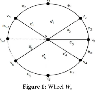
A wheel Wn is the join of Cn and K1. Clearly Wn has n+1 vertices and 2n edges. A wheel Wn is shown in Figure 1. The vertices Cn are called rim vertices and the vertex of K1 is called apex.

Figure 1: Wheel Wn

Lemma 2. Let Wn be a wheel with 2n edges, n≥3. Then

4

Theorem 3. Let Wn be a wheel with n+1 vertices and 2n edges, n ≥ 3. Then

(i)

( )

2 _{2 18}.

2 9 n n n SKB W n n n = + + + +

(ii)

( )

( ₁)( ₉) 9.

n

n n

PKB W

n

n n n

= +

+

+ +

(iii)

( )

( )( )

2

2 7 2 16

.

1 9 9

n

n n n n

ABCKB W n

n n n n

+ + +

= +

+ + +

(iv)

( )

2 ₂( 1)( 9) .

2 9

n

n n n n

GAKB W n

n n

+ +

= +

+ +

(v) RKB W

( )

n =n n2+2n+ +9 n n( +9 .)

Proof: Let Wn be a wheel with n+1 vertices and 2n edges. By using definitions and Lemma 2, we obtain

(i)

( )

( ) ( )

( )

1

n

n

uv E W _{e e}

SKB W

S u S v

∈ =

+

∑

( 1) 9 9 9

n n

n n

n n n

= +

+ + + + + +

2 _{2 18}.

2 9 n n n n n = + + + +

(ii)

( )

( ) ( )

( )

1

n

n

uv E W _{e e}

PKB W

S u S v

∈

=

∑

( 1)( 9) ( 9)( 9)

n n

n n n n n

= +

+ + + +

( ₁)( ₉) 9.

n n

n

n n n

= +

+

+ +

(iii)

( )

( ) ( )

( ) ( ) ( ) 2 n e e n

uv E W e e

S u S v ABCKB W

S u S v

∈

+ −

=

∑

( )

( 11)( 99)2 ( 91)( 99)2

n n n n n

n n

n n n n n

+ + + − + + + −

= +

+ + + +

( )( ) ( )

2

2 7 2 16

.

1 9 9

n n n

n n

n n n n

+ + +

= +

+ + +

(iv)

( )

( ) ( )

( ) ( ) ( ) 2 n e e n

uv E W e e

S u S v GAKB W

S u S v

∈ =

+

∑

2 ₍ ( _{) (}1)( 9₎) 2₍ ( _{) (}9)( 9₎)

1 9 9 9

n n n n n n n

n n n n n

+ + + +

= +

+ + + + + +

( )( )

2

2 1 9

.

2 9

n n n n

n n n

+ +

= +

+ +

(v)

( )

( ) ( )

( )n

n e e

uv E W

RKB W S u S v

∈

=

∑

=n n n( +1)(n+9)+n (n+9)(n+9)

( )

2

2 9 9 .

n n n n n

5 4. Results for gear graphs

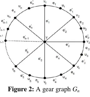
A gear graph is obtained from Wn by adding a vertex between each pair of adjacent rim vertices and it is denoted by Gn. Clearly Gn has 2n+1 vertices and 3n edges. A graph Gn is shown in Figure 2.

Figure 2: A gear graph Gn

Lemma 4. Let Gn be a gear graph with 2n+1 vertices and 3n edges. Then Gn has two types of edges as follows:

E1={uv ∈ E(Gn)| Se(u) = n (n+1), Se(v) = n+7}, | E1 | = n. E2={uv ∈ E(Gn)| Se(u) = n+7 , Se(v) = 6}, | E2 | = 2n.

Theorem 5. Let Gn be a gear graph with 2n + 1 vertices 3n edges. Then

(i)

( )

2

2 . 13

2 7

n

n n

SKB G

n n n

= +

+

+ +

(ii)

( )

( )( ) ( )

2 .

1 9 6 7

n

n n

PKB G

n n n n

= +

+ + +

(iii)

( )

( )( ) ( )

1 1

2 ₂

2

2 5 11

2 .

1 7 6 7

n

n n n

ABCKB G n n

n n n n

 _{+ +}   ₊ 

=   +  

+ + +

   

(iv)

( )

2 ₂( 1)( 7) 4 6( 7).

2 7 13

n

n n n n n n GAKB G

n n n

+ + +

= +

+ + +

(v) RKB G

( )

n =n n n( +1)(n+7)+2n 6(n+7 .)

Proof: Let Gn be a gear graph with 2n+1 vertices and 3n edges. By using definitions and Lemma 4, we obtain

(i)

( )

( ) ( )

( )

1

n

n

uv E G

e e

SKB G

S u S v

∈ =

+

∑

( ) ( )

2 7 6

1 7

n n

n

n n n

= +

+ + + + +

2

2 . 13

2 7

n n

n n n

= +

+

+ +

(ii)

( )

( ) ( )

( )

1

n

n

uv E G _{e e}

PKB G

S u S v

∈

=

∑

( )( ) ( )

2

1 7 6 7

n n

n n n n

= +

6

(iii)

( )

( ) ( )

( ) ( )

( )

2

n

e e

n

uv E G e e

S u S v ABCKB G

S u S v

∈

+ −

=

∑

( ) ( )

( )( ) ( )

1 1

2 2

1 7 2 7 6 2

2

1 7 7 6

n n n n

n n

n n n n

 _{+ + + −}   _{+ + −} 

=   +  

+ + +

   

( )( ) ( )

1 1

2 ₂

2

2 5 11

2 .

1 7 6 7

n n n

n n

n n n n

 _{+ +}   ₊ 

=   +  

+ + +

   

(iv)

( )

( ) ( )

( ) ( )

( )

2

n

e e

n

uv E G e e

S u S v GAKB G

S u S v

∈ =

+

∑

2 ₍ ( ₎1)( 7) 2 2 ( 7 6)

1 7 7 6

n n n n n n

n n n n

+ + +

= +

+ + + + +

( )( ) ( )

2

2 1 7 4 6 7

2 7 13

n n n n n n

n n n

+ + +

= +

+ + +

(v)

( )

( ) ( )

( )n

n e e

uv E G

RKB G S u S v

∈

=

∑

=n n n( +1)(n+7)+2n 6(n+7 .)

( )

2

2 9 2 6 7 .

n n n n n

= + + + +

5. Results for helm graphs

A helm graph Hn is a graph obtained from Wn by attaching an end edge to each rim vertex. Clearly Hn has 2n+1 vertices and 3n edges. A graph Hn is depicted in Figure 3.

Figure 3: A graph Hn

Lemma 6. If Hn is a helm graph with 2n+1 vertices and 3n edges, then Hn has three types of edges as

E1={uv ∈ E(Hn)| Se(u) = n(n+2), Se(v) = n + 17} | E1 | = n. E2={uv ∈ E(Hn)| Se(u) = Se(v) = n + 17}, | E2 | = n. E3={uv ∈ E(Hn)| Se(u) = n +17, Se(v) = 3} | E3 | = n.

Theorem 7. If Hn is a helm graph with 2n+1 vertices and 3n edges, then

(i)

( )

2 _{2 34 20}.

3 17

n

n n n

SKB H

n n n n

= + +

+ +

7

(ii)

( )

( ₂)( ₁₇) ( 17) ₃( ₁₇).

n

n n n

PKB H

n

n n n n

= + +

+

+ + +

(iii)

( )

( )( ) ( )

1 1

2 ₂

2

3 5 2 32 18

.

2 17 17 3 17

n

n n n n

ABCKB H n n n

n n n n n

 _{+ +}  ₊  ₊ 

=   + +  

+ + + +

   

(iv)

( )

2 ₂( 1)( 7) 2 3( 17).

3 7 20

n

n n n n n n

GAKB H n

n n n

+ + +

= + +

+ + +

(v) RKB H

( )

_n =n n n( +2)(n+17)+n n( +17)+n 2(n+17 .)

Proof: Let Hn be a helm graph with 2n+1 vertices and 3n edges. Then by using definitions and Lemma 6, we deduce

(i)

( )

( ) ( )

( )

1

n

n

uv E H _{e e}

SKB H

S u S v

∈ =

+

∑

( )

2

17 17 17 3

2 17

n n n

n n n

n n n

= + +

+ + + + +

+ + +

2 _{2 34 20}.

3 17

n n n

n n n n

= + +

+ +

+ +

(ii)

( )

( ) ( )

( )

1

n

n

uv E H _{e e}

PKB H

S u S v

∈

=

∑

( 2)( 17) ( 17)( 17) ( 17 3)

n n n

n n n n n n

= + +

+ + + + +

( ₂)( ₁₇) ( 17) ₃( ₁₇).

n n n

n

n n n n

= + +

+

+ + +

(iii)

( )

( ) ( )

( ) ( )

( )

2

n

e e

n

uv E H e e

S u S v ABCKB H

S u S v

∈

+ −

=

∑

( )

( )( ) ( )( )

1 2

2 17 2 17 17 2

2 17 17 17

n n n n n

E E

n n n n n

+ + + − + + + −

= +

+ + + +

( )

3

17 3 2

17 3

n n

E

n

+ + + − +

+

( )( ) ( )

1 1

2 ₂

2

3 15 2 32 18

.

2 17 17 3 7

n n n n

n n n

n n n n n

 _{+ +}  ₊  ₊ 

=   + +  

+ + + +

   

(iv)

( )

( ) ( )

( ) ( )

( )

2

n

e e

n

uv E H e e

S u S v GAKB H

S u S v

∈ =

+

∑

( )( )

( )

( )( )

1 2

2 2 17 2 17 17

2 17 17 17

n n n n n

E E

n n n n n

+ + + +

= +

8

( )

3

2 17 3

17 3

n E

n

+ +

+ +

( )( ) ( )

2

2 2 7 2 3 17

. 20 3 17

n n n n n n

n n

n n

+ + +

= + +

+

+ +

(v)

( )

( ) ( )

( )n

n e e

uv E H

RKB H S u S v

∈

=

∑

( )( ) ( )( ) ( )

1 2 17 2 17 17 3 17 3.

E n n n E n n E n

= + + + + + + +

( 2)( 17) ( 17) 3( 17 .)

n n n n n n n n

= + + + + + +

Acknowledgement. The author is thankful to the referee for his/her suggestions. REFERENCES

1. V.R.Kulli, College Graph Theory, Vishwa International Publications, Gulbarga, India (2012).

2. I.Gutman and O.E.Polansky, Mathematical Concepts in Organic Chemistry, Springer, Berlin (1986).

3. V.R.Kulli, Multiplicative Connectivity Indices of Nanostructures, LAP LEMBERT Academic Publishing (2018).

4. B.Basavanagoud, P.Jakkannavar, Kulli-Basava indices of graphs, Inter. J. Appl. Engg. Research, 14(1) (2018) 325-342.

5. V.R.Kulli, Some new topological indices of graphs, International Journal of Mathematical Archive, 10(5) (2019) 62-70.

6. V.R.Kulli, Product connectivity leap index and ABC leap index of helm graphs, Annals of Pure and Applied Mathematics, 18(2) (2018) 189-193.

7. V.R.Kulli, The sum connectivity Revan index of silicate and hexagonal networks, Annals of Pure and Applied Mathematics, 14(3) (2017) 401-406.

8. V.R.Kulli, Computing reduced connectivity indices of certain nanotubes, Journal of Chemistry and Chemical Sciences, 8(11) (2018) 1174-1180.

9. V.R.Kulli, Degree based connectivity F-indices of dendrimers, Annals of Pure and Applied Mathematics, 18(2) (2018) 201-206.