ESAIM: PROCEEDINGS,December 2012, Vol. 38, p. 99-117
F. Coquel, M. Gutnic, P. Helluy, F. Lagouti`ere, C. Rohde, N. Seguin, Editors
NUMERICAL SIMULATION OF THE SELECTION PROCESS OF THE
OVARIAN FOLLICLES
Benjamin Aymard
1,2, Fr´
ed´
erique Cl´
ement
2, Fr´
ed´
eric Coquel
3and Marie
Postel
1Abstract. This paper presents the design and implementation of a numerical method to simulate a multiscale model describing the selection process in ovarian follicles. The PDE model consists in a quasi-linear hyperbolic system of large size, namely Nf×Nf, ruling the time evolution of the cell
density functions ofNf follicles (in practice Nf is of the order of a few to twenty). These equations
are weakly coupled through the sum of the first order moments of the density functions. The time-dependent equations make use of two structuring variables, age and maturity, which play the roles of space variables. The problem is naturally set over a compact domain of R2. The formulation of the time-dependent controlled transport coefficients accounts for available biological knowledge on follicular cell kinetics. We introduce a dedicated numerical scheme that is amenable to parallelization, by taking advantage of the weak coupling. Numerical illustrations assess th e relevance of the proposed method both in term of accuracy and HPC achievements.
R´esum´e. Ce document pr´esente la conception et l’impl´ementation d’une m´ethode num´erique servant `
a simuler un mod`ele multi´echelle d´ecrivant le processus de s´election des follicules ovariens. Le mod`ele EDP consiste en un syst`eme hyperbolique quasi lin´eaire de grande taille, typiquementNf×Nf,
gou-vernant l’´evolution des fonctions de densit´e cellulaire pourNf follicules (en pratiqueNf est de l’ordre
de quelques-uns `a une vingtaine). Ces ´equations d’´evolution utilisent deux variables structurantes, l’ˆage et la maturit´e, qui jouent le rˆole de variables d’espace. Le probl`eme est naturellement pos´e sur un domaine compact de R2. La formulation du transport `a coefficients variables au cours du temps en fonction du contrˆole est issue des connaissances disponibles sur la cin´etique cellulaire au sein des follicules ovariens. Nous pr´esentons un sch´ema num´erique d´edi´e au probl`eme parall´elisable en tirant parti du faible couplage. Des simulations num´eriques permettent d’´evaluer la pertinence de la m´ethode propos´ee tant en terme de pr´ecision que de calcul haute performance.
Introduction
This work is motivated by a mathematical modelling approach of a complex physiological system, the develop-ment of ovarian follicles. The model describes both the cell dynamics within each follicle and the competition process within the population of follicles. The resulting model ( [9]) is a large scale system of weakly coupled quasi-linear transport equations, where integro-differential terms occur both in the velocity and source term. The coupling terms account for the endocrine-based dependence of one follicle dynamics on all other developing
1 UPMC Univ Paris 06, UMR 7598, Laboratoire Jacques-Louis Lions, F-75005, Paris, France
CNRS, UMR 7598, Laboratoire Jacques-Louis Lions, F-75005, Paris, France
2 Centre de Recherche INRIA Paris-Rocquencourt, Domaine de Voluceau, B.P. 105 - F-78153 Le Chesnay, France 3 CMAP, Ecole Polytechnique, CNRS, route de Saclay, F-91128 Palaiseau C´edex-France
c
EDP Sciences, SMAI 2012
follicles. The well-posedness of the Cauchy problem is established in [15]. Existence and uniqueness of weak solutions is proved for bounded initial conditions. The competition process was investigated in a game theory approach after reducing the PDE model to coupled ODE systems [14]. Control problems associated with this model are investigated in [8] (computation of backwards reachability sets) and [4] (optimal control in minimal time).
We are specifically interested in the numerical issues raised by this multiscale model. In previous works [3, 7], a CTU numerical scheme has been implemented in the Bearclaw1environment, which is based on adaptive mesh refinement using wave-propagation algorithms [12, 13]. Here, we develop a dedicated code, which allows us (i) to handle the conservative form of the equations, (ii) to deal with the discontinuous coefficients and (iii) to use high performance computing (HPC) techniques in order to speed up the computing and be able to simulate as many as twenty follicles.
The paper is organized as follows. In section 1, we introduce the biological background and the multiscale model. In section 2, we describe the numerical scheme in detail. In section 3, we illustrate the simulation outputs and assess the algorithm robustness, accuracy and scalability on parallel architectures.
1.
Biological and biomathematical background
1.1.
Biological background
FSH
pituitary gland
oocyte theca layer
granulosa layer
antrum
ovary follicle estradiol inhibin
Differentiation Proliferation
Apoptosis
gonadal axis
Macroscopic scale: Mesoscopic scale: ovarian follicle Microscopic scale: granulosa cell
hypothalamo pituitary
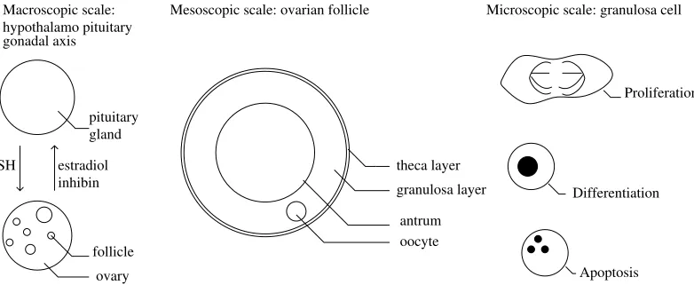
Figure 1. Follicle development as a multiscale process. Left : endocrine feedback loop between the ovaries and the hypothalamo-pituitary-axis. Middle : schematic 2D view of an ovarian follicle. Right : different cell states encountered by the granulosa cells during follicular devel-opment.
1.1.1. Mesoscopic scale: ovarian follicles
Ovarian follicles are spheroidal tissular structures sheltering the oocytes (figure 1). Each follicle goes through a development process, composed of two main parts : the basal development and the terminal development (figure 2). During basal development, the follicles are independent of hormonal support from the pituitary gland, while, during the terminal part of their development, they become dependent on FSH (follicle stimulating hormone) supply. Follicle development can end up either by ovulation, in the best case, or much more often by degeneration through atresia. The commitment of a follicle to either ovulation or atresia is driven by the changes occurring in the follicular cell population.
1http://www.pas.rochester.edu/˜bearclaw/
follicle
Antrum follicle Primordial
Preovulatory follicle granulosa
layer
granulosa layer Basal development Terminal development
Atresia Ovulation
Figure 2. Follicular development : from basal to terminal development. After exiting the pool of quiescent primordial follicles, ovarian follicles enter a several-month long process of growth and maturation, that either ends up by ovulation or degeneration through atresia. In the basal part of development, follicle growth is mainly due to the oocyte enlargement and increase in the number of granulosa cell layers. In the final part of development, granulosa cells progressively stop proliferating and follicle growth is mainly due to the enlargement of the antrum, a liquid-filled cavity in the center of the follicle.
1.1.2. Macroscopic scale : competition process and endocrine feedback loop
In some sense, the terminal part of follicle development can be considered as a competition between follicles for FSH resource. FSH controls follicle development, while FSH levels are in turn controlled by two hormones secreted by the ovary, inhibin and estradiol, whose plasma levels are determined by the summed contributions of all maturing follicles (figure 1). This ovarian hormonal feedback induces a drop in FSH levels that will penalize the follicles, except those (in the poly-ovulating situations) or that (in the mono-ovulating ones) that are sufficiently mature to survive in a FSH poor environment. The rising levels of estradiol finally triggers the ovulatory surge that leads to the ovulation of the surviving follicles.
1.1.3. Microscopic scale : granulosa cell kinetics
Each granulosa cell can be encountered in either of three different cell states : proliferation, differentiation or apoptosis (programmed cell death) (figure 3). At the beginning of terminal development, most granulosa cells are progressing along the cell division cycle, that can be split into aG1 phase, where cells are sensitive to FSH control, and a SM phase, where cells are preparing for mitosis and are insensitive to FSH control. At the end of mitosis, one single mother cell gives birth to two daughter cells. During the FSH sensitive phase, cells become more and more mature, up to a point where they reach a threshold maturity and exit the cell division cycle. At this time they are exposed to a great risk of apoptosis, and may die if the FSH environment is not favorable. After exiting the cell cycle, the cells stop proliferating definitively, but their maturity still increases, so that they contribute more and more to hormone (and especially estradiol) secretion.
1.2.
Biomathematical model
1.2.1. Computing domain
Let us introduce the variables
a age,
γ maturity, t time,
the vector of granulosa cell densities for theNf follicles
Φ(a, γ, t) = (φ1(a, γ, t), ..., φNf(a, γ, t)),
and the computing domain Ω in the (a, γ) plane,
Ω ={(a, γ),0≤a≤Nc×Da,0≤γ≤1}
where Nc is the number of cell cycles andDa is the duration of one cycle. The different cell states described
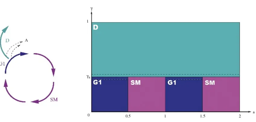
in paragraph 1.1.3 take place in three subdomains as illustrated in Figure 3. The differentiation phase D corresponds to the area of the domain where the maturity overcomes the cellular maturity thresholdγs
G1 ={(a, γ)∈Ω, pDa≤a≤(p+ 1/2)Da, p= 0, . . . , Nc−1, 0≤γ≤γs},
SM={(a, γ)∈Ω, (p+ 1/2)Da ≤a≤(p+ 1)Da, p= 0, . . . , Nc−1, 0≤γ≤γs},
D={(a, γ)∈Ω, γs≤γ}.
Figure 3. Division of the spatial domain according to the cell phases for unit cycle duration Da = 1. Left : schematic view of a granulosa cell cycle. Right : (a, γ)plane. The bottom part
represents the successive cell cycles, each composed of the G1 and SM phases. The top part corresponds to the differentiation phase.
1.2.2. Hyperbolic system
If we consider, for each follicle, a conservation law for the granulosa cell population density, we obtain the following hyperbolic system, satisfied by Φ:
∂φ1(a, γ, t)
∂t +
∂(g(a, γ, u1(t))φ1(a, γ, t))
∂a +
∂(h(a, γ, u1(t))φ1(a, γ, t))
∂γ =−λ(a, γ, U(t))φ1(a, γ, t) ..
. ∂φf(a, γ, t)
∂t +
∂(g(a, γ, uf(t))φf(a, γ, t))
∂a +
∂(h(a, γ, uf(t))φf(a, γ, t))
∂γ =−λ(a, γ, U(t))φf(a, γ, t) ..
. ∂φNf(a, γ, t)
∂t +
∂(g(a, γ, uNf(t))φNf(a, γ, t))
∂a +
∂(h(a, γ, uNf(t))φNf(a, γ, t))
∂γ =−λ(a, γ, U(t))φNf(a, γ, t)
(1) The initial condition is given by the distribution of the granulosa cell populations at the initial time
Φ(a, γ,0) = Φ0(a, γ)
where Φ0 is compactly supported in ]0, NcDa[×]0,1[. Since the functional domain Ω is compact, we need to
express boundary conditions. Considering some qualitative properties of the maturation function h, defined below, the horizontal top boundaryγ= 1 is never reached. Similarly, we can fix the number of cell cyclesNc in
accordance with the ageing functiong, so that the right vertical boundarya=NcDais never reached. For sake
of computing simplicity, we therefore assume spatial periodicity on the outer boundaries of Ω in the numerical simulations.
The ageing functiong appearing in (1) is defined by
g(a, γ, u) =
g1u+g2 for (a, γ)∈G1
1 for (a, γ)∈SM∪D (2)
whereg1, g2 are real positive constants. The maturation functionhis defined by
h(a, γ, u) =
(
τh(−γ2+ (c1γ+c2)(1−exp(
−u ¯
u ))) for (a, γ)∈G1∪D
0 for (a, γ)∈SM
(3)
whereτh,c1,c2and ¯uare real positive constants. The source term, that represents cell loss through apoptosis, is defined by
λ(a, γ, U) =
Kexp(−((γ−γs) 2
¯
γ ))×(1−U) for (a, γ)∈G1∪D
0 for (a, γ)∈SM
(4)
whereK,γsand ¯γ are real positive constants.
Remark. The precise values of the constants depends on species and breeds; they will be fixed later.
1.2.3. Closure equations
The equations in the PDE system (1) are linked together through the argument uf(t) appearing in the speeds
g(a, γ, uf) and h(a, γ, uf) and the argument U(t) in the source term λ(a, γ, U). U(t) and uf(t) represent
respectively the plasma FSH level and the locally bioavailable FSH level and depend on some maturation moments of the densities.
• follicular cell mass (local, one by follicle)
m0(f, t) = Z 1
0 Z NcDa
0
φf(a, γ, t)dadγ, 1≤f ≤Nf (5)
This moment is an interesting quantity since it corresponds to an observable variable (the total cell number in one follicle) even if it does not come as such into play in the equations.
• follicular maturity (local, one by follicle)
m(f, t) =
Z 1
0 Z NcDa
0
γφf(a, γ, t)dadγ, 1≤f ≤Nf (6)
• ovarian maturity (global, shared by all follicles)
M(t) =
Nf X
f=1
m(f, t), (7)
• plasma FSH level (global, shared by all follicles)
U(t) =Umin+
1−Umin
1 + exp(c(M(t)−M¯)), (8)
whereUmin,c and ¯M are real positive constants
• locally bioavailable FSH level
uf(t) = min
b1+
eb2m(f,t)
b3
,1
U(t), (9)
whereb1, b2 andb3 are real positive constants.
It is important to notice that the ageing function (2) is discontinuous (in general) on the interfacesG1−SM, and that the maturation function (3) is discontinuous (in general) on the interfaces SM−D (Figure 3). It is necessary to introduce transmission conditions in order to overcome possible failure of uniqueness due to the discontinuities in coefficients (see [10] or [1] for instance). The precise definition of the required transmission conditions has been addressed in the paper by Peipei Shang ( [15]). We suppose that, for each cyclep= 1, . . . , Nc
and each folliclef = 1, . . . , Nf, the flux on thea-axis is continuous between the phasesG1 andSM
φf(t, a+, γ) = (g1uf +g2)φf(t, a−, γ), a= (p−1/2)Da, 0≤γ≤γs, (10)
and that the flux is doubling on the interfacesSM−G1, which accounts for the birth of new cells at the end of each cell cycle
(g1uf+g2)φf(t, a+, γ) = 2φf(t, a−, γ), a=pDa, 0≤γ≤γs. (11)
Finally, we suppose homogeneous Dirichlet condition to the north of the interfaceSM−D
φf(t, a, γs+) = 0, (p−1/2)Da≤a≤pDa. (12)
The time dependent ovarian maturityM(t) defined in (7) is compared to the ovarian maturity threshold, denoted byMo, to define the final time, beyond which the competition is over
tf inal= inf{t, M(t)≥Mo}. (13)
The follicles are then sorted into two classes : ovulatory if the maturity is higher than the follicle maturity threshold, denoted byMf, atretic otherwise.
2.
Numerical Method
2.1.
Discretization
In this paragraph the cycle duration is set to Da = 1. We denote by ∆a (respectively ∆γ ) the space step
in the age (respectively maturity) direction. In practice we choose ∆a = ∆γ. The discretization step ∆γ
and the cellular maturity thresholdγs must be chosen so that the interfaces where the speed coefficients (2,3)
are discontinuous fall on grid points covering the computational domain of size [Nc,1]. Denoting by Nm the
number of grid cells by half granulosa cell cycle, we setNγ = 2Nmand ∆a= ∆γ= 1/Nγ and we introduce the
dedicated2notations for grid points (a
k, γl) and mesh centers (ak+1/2, γl+1/2)
ak =k∆a, ak+1/2= (k+ 1/2)∆a, fork= 0, . . . , Nc×Nγ, (14)
γl=l∆γ, γl+1/2= (l+ 1/2)∆γ, forl= 0, . . . , Nγ. (15)
Considering that the time step ∆tn may change at every iteration, in order to preserve stability, the time
discretization is defined by
t0= 0, tn+1=tn+ ∆tn, forn= 0, . . . , Nt (16)
with Ntsuch that tNt =tfinal. The unknowns are the approximate mean values of the density vector in each
grid mesh
Φnk,l≈ 1 ∆a∆γ
Z ak+1
ak
Z γl+1
γl
Φ(a, γ, tn)dγda, for k= 0, ..., NcNγ−1, andl= 0, ..., Nγ−1
whose components φn
f,k,l are the discrete density values for each follicle.
2.2.
Macroscopic scale : piecewise constant approximation of the hormonal control
We define the approximation of the control terms (5 - 9) at each time stepn= 0, . . . , Nt
mn0,f = ∆a∆γ
Nγ−1 X
l=0
NcNγ−1 X
k=0
φnf,k,l, forf = 1, . . . , Nf, (17)
mnf = ∆a∆γ Nγ−1
X
l=0
γl+1/2 NcNγ−1
X
k=0
φnf,k,l, forf = 1, . . . , Nf, (18)
Mn =
Nf X
f=1
mnf, (19)
Un = Umin+
1−Umin
1 + exp(c(Mn−M¯)), (20)
unf = min(b1+
eb2mnf
b3
,1)Un, forf = 1, . . . , Nf. (21)
2.3.
Mesoscopic scale : finite volume scheme
We use a splitting strategy in order to compute the solution of the PDE system (1), which amounts to a convective equation combined with a source equation, for each folliclef = 1, . . . , Nf
∂tφf(a, γ, t) +∂a(g(a, γ, uf(t))φf(a, γ, t)) +∂γ(h(a, γ, uf(t))φf(a, γ, t)) = 0 (convective part), (22)
∂tφf(a, γ, t) =−λ(a, γ, U(t))φf(a, γ, t) (source part). (23)
2We use this index notation for the use of the forthcoming Multiresolution development
2.3.1. Convective part
The convection part (22) is treated with a classical finite volume method. The approximate mean values of the solution att= 0 are initialized using a midpoint formula, accurate at the order 2 in space
Φ0k,l= Φ0(ak+1/2, γl+1/2).
Using the integral form of the conservation law
Z tn+1
tn
Z ak+1
ak
Z γl+1
γl
(∂tφf(a, γ, t) +∂a(g(a, γ, uf(t))φf(a, γ, t)) +∂γ(h(a, γ, uf(t))φf(a, γ, t)))dγdadt= 0,
we obtain a recursion on the approximate density of each follicle, where we drop the indexf for clarity sake
φnk,l+1=φnk,l− ∆t ∆a
Gk+1,l+1 2(Φ
n)−G k,l+1
2(Φ
n)− ∆t
∆γ
Hk+1 2,l+1(Φ
n)−H k+1
2,l(Φ
n) (24)
whereGk,l+1
2 (respectivelyHk+ 1
2,l) is the numerical flux across the vertical edge [(ak, γl),(ak, γl+1)] (respectively
the horizontal edge [(ak, γl),(ak+1, γl)]) defined by
Gk,l+1 2(Φ
n)≈ 1
∆tn∆γ Z tn+1
tn
Z γl+1
γl
g(ak, γ, uf(t))φ(ak, γ, t)dγdt,
Hk+1 2,l(Φ
n)≈ 1
∆tn∆a Z tn+1
tn
Z ak+1
ak
h(a, γl, uf(t))φ(a, γl, t)dadt.
(25)
The dependence of the flux functions on all the follicle densities through the control termuf is emphasized by
the Φn argument. It appears in the explicit in time approximations of the speeds (2), and (3) at the center of the mesh
(
gn
k,l=g(ak+1 2, γl+
1 2, u
n f),
hn
k,l=h(ak+1 2, γl+
1 2, u
n f).
Note that the transmission conditions (10) and (11) on the interfaces where these speed coefficients (2) and (3) are discontinuous are exactly treated with the method described in the article of Godlewski and Raviart ( [10]). The numerical fluxes (25) are designed using a limiter strategy. Indeed, it is well known that first order schemes, like the Godunov scheme, are diffusive, and that second order schemes, like Lax Wendroff scheme, generate oscillations in the neighborhood of discontinuities. In order to get a stable as well as precise scheme, we take a weighting of a low order scheme and a high order scheme, and we define limited numerical fluxes
G=GLow+`(rG)(GHigh−GLow),
H =HLow+`(rH)(HHigh−HLow), (26)
where` is a limiter function, for example van Leer function
`(r) = r+|r| 1 +r
andrG, rH are
rG =
gk−1,lφk−1,l−gk−2,lφk−2,l
gk,lφk,l−gk−1,lφk−1,l
if gk−2,l ≥0 and gk−1,l≥0 and gk,l≥0,
gk+1,lφk+1,l−gk,lφk,l
gk,lφk,l−gk−1,lφk−1,l
if gk−1,l≤0, and gk,l≤0 and gk+1,l≤0,
0 otherwise,
rH =
hk,l−1φk,l−1−hk,l−2φk,l−2
hk,lφk,l−hk,l−1φk,l−1
if hk,l−2≥0 and hk,l−1≥0 and hk,l≥0,
hk,l+1φk,l+1−hk,lφk,l
hk,lφk,l−hk,l−1φk,l−1
if hk,l−1≤0 and hk,l≤0 and hk,l+1≤0,
0 otherwise.
These ratios are good indicators of the regularity of the function in each direction (see [16]). In fact, a steep gradient or a discontinuity gives a ratio far from 1, whereas a smooth function gives a ratio close to 1.
The first order fluxes entering equation (26) are the Godunov fluxes
GLowk,l+1 2
(Φn) = (gnk−1,l)+φkn−1,l+ (gnk,l)−φnk,l,
HLow k+1 2,l
(Φn) = (hn k,l−1)
+φn
k,l−1+ (h n k,l)
−φn k,l,
and the high order fluxes are the Lax Wendroff ones
GHighk,l+1 2
(Φn) = 1
2(g
n k−1,lφ
n k−1,l+g
n k,lφ
n k,l),
HkHigh+1 2,l
(Φn) = 1
2(h
n k,l−1φ
n k,l−1+h
n k,lφ
n k,l).
Consequently, since ∆a= ∆γ, the CFL condition which guarantees the stability is
∆tnf,F V S≤CF L ∆γ
maxk,l(|gk,l|,|hk,l|)
(27)
withCF L≤ 1 2.
2.3.2. Source part
The source part (23) of the PDE system is explicitly dealt with
φnk,l+1=φnk,l−∆tλ(ak+1 2, γl+
1 2, U
n)φn
k,l, (28)
which implies a stability condition on the time step, which we strengthen to enforce positivity
∆tnf,source≤ 1 maxk,l|λ(ak+1
2, γl+ 1 2, U
n)|. (29)
2.4.
Macro/Meso scale Parallelization
In order to speed up the numerical simulations, the code is implemented on a parallel architecture. Every follicle follows its own dynamic independently of the others, except that it shares with them the FSH resource, and that it contributes to the tuning of plasma FSH level. Hence it is natural to use a SIMD (single instruction, multiple data) strategy, with one follicle by process. The only communications that have to be done at each time step concern the ovarian maturity, through a reduction operation (sum) and the current time step ∆tn,
through a reduction operation (min). Each process computes the maximum time step satisfying both conditions (27) and (29)
∆tnf = min{∆tnf,F V S,∆tnf,source} (30)
relevant for its own follicle, and the time step used by all processes is
∆tn = min
f {∆t n
f}. (31)
2.5.
Parallel algorithm and improvement to order
2
in time
Finally, we get the following parallel algorithm for each time step:
(1) Compute time step
• Compute local time step ∆tn f (30)
• Communication: Compute the minimum of local time steps ∆tn (31)
(2) Update solution
• Flux computation (26), • Convection computation (24), • Source computation (28), (3) Update control terms
• Compute local maturity (18),
• Communication: compute the sum of local maturities (19), • Compute FSH plasma level (20),
• Compute locally bioavailable FSH rate (21).
Denoting byE the evolution operator, that consists in steps (2) and (3), the second order in time is achieved by a second order Runge-Kutta method (Heun)
φ∗ = E(φn),
φ∗∗ = E(φ∗),
φn+1 = 1 2(φ
n+φ∗∗).
3.
Numerical simulations
The code was developed in C++ using the parallel library MPI. The tests were performed on the Jacques-Louis Lions Laboratory super calculator SGI Altix UV 100. The current configuration is 64-core 2 GHz. The visualizations were made with OpenGL and gnuplot.
3.1.
Initial condition
In the first test case, we used, for sake of comparison with anterior results, a piecewise constant function similar to the initial condition used in [7, 8]. Its support in age covers the first cycle while its amplitude is a step-decreasing function of the maturity.
φ0(a, γ) =
8 if 0.05≤γ <0.1 7 if 0.1≤γ <0.15 5 if 0.15≤γ <0.2 0 otherwise.
if 0≤a≤1,
0 otherwise.
(32)
For the other test cases we used as initial condition a gaussian function centered inC= (Ca, Cγ)
φ0(a, γ) = 1 2πσexp
1
2
(a−C a)2
σ2 +
(γ−Cγ)2
σ2
. (33)
The varianceσ2 can be chosen so thatφ
0be smooth enough to be used for testing the convergence rate, which is checked in the paragraph 3.5.
3.2.
Sets of default parameters
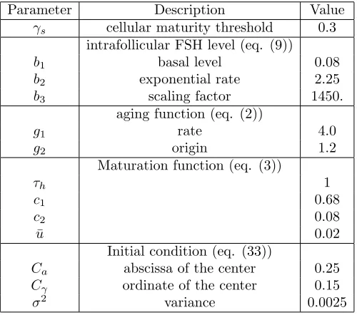
Since one of our goals was to improve the computational method, we used the same set of parameters as in [8] to be able to compare at least qualitatively our results to previous simulation outputs. We distinguished two sets of parameters, one, in Table 1, for theglobalparameters, that are identical for all follicles (space discretization, CFL condition,. . . ), another, in Table 2, for the local parameters (initial condition, velocity parameters,. . . ), which can depend on the follicle.
Parameter Description Value
Nm number of grid cells by half granulosa cell cycle 30
Nc number of cycles 8
CFL CFL condition 0.4
Mf follicular maturity threshold 0.7
Mo ovarian maturity threshold 5.
FSH plasma level (eq. (8))
Umin minimum level 0.075
c slope parameter 2.0
¯
M abscissa of the inflection point 4.5
Apoptosis source term (eq. (4))
K intensity factor 6.0
¯
γ scaling factor 0.02
tmax maximum time (to avoid excessively long computations) 7
Table 1. Values of the global parameters used in Figures 4 to 9
. The number of follicles,Nf, and the number of grid cells by half granulosa cell cycle,Nm, may depend on the
simulation.
Parameter Description Value
γs cellular maturity threshold 0.3
intrafollicular FSH level (eq. (9))
b1 basal level 0.08
b2 exponential rate 2.25
b3 scaling factor 1450.
aging function (eq. (2))
g1 rate 4.0
g2 origin 1.2
Maturation function (eq. (3))
τh 1
c1 0.68
c2 0.08
¯
u 0.02
Initial condition (eq. (33))
Ca abscissa of the center 0.25
Cγ ordinate of the center 0.15
σ2 variance 0.0025
Table 2. Values of the local (follicle-dependent) parameters used in Figures 4 to 9
3.3.
Time evolution of the cell density for one follicle
We have first studied the behavior of the cell density of one single follicle as a function of time, in order to check some qualitative properties.
The full movie can be downloaded from http://www.ljll.math.upmc.fr/aymard/CEMRACS2011.gif and four snapshots are displayed on Figure 4. Note that on the snapshots the color code is time dependent while in the movie it is set once and for all at initial time.
The parameters values are gathered in Table 1 and 2, except for g2 = 1.2 and τh = 1.2. Also, in this
mono-ovulatory situation we set the follicular and ovarian maturity thresholds equal toMo=Mf = 16.5. The spatial
discretization for this test uses Nm= 30 cells per half granulosa cell cycle, and the domain Ω contains eight
cycles. The grid size is therefore 8×(2×30)2= 28800.
On the first snapshot 4 a), we can observe the piecewise constant initial condition (32). The cell mass is equal to 1.
On the second snapshot 4 b), at time 0.91, we can see that the density has moved to the second cycle. The cell mass is equal to 2.17. At the interfacea= 2.5 between zoneG1 andSM the ageing function decreases, which results in a local increase in the density, whose profile becomes narrower. The cell density is starting to double at the end of the second cell cycle, on the SM-G1 interface at a= 3.
On the third snapshot 4 c), at time 1.57, the cell density has reached the third cycle. It is splitting into a fully differentiated subpopulation and a still proliferating one. It is worth noticing that, consistently with the model, there is no crossing of the SM-D interface. The cell mass is equal to 3.7.
On the last snapshot 4 d), around timet= 5, towards the end of the simulation, the density is concentrated in theD phase above the seventh cell cycle. Even if all cells have exited the cell cycle, we can distinguish three different density clouds, each of which being issued from one of the previous cycles. The cell mass is equal to 14.7.
In Figure 5 the time evolution of the cell mass (panel A) and follicular maturity (panel B) are displayed as green curves. While the cell mass reaches a constant value as soon as all cells have entered the differentiating phase, the maturity goes on increasing. The blue curves correspond to a similar simulation with a slower maturation function, whereτh= 1 instead of 1.2. The cells spend more time in the proliferating phase and they enter the
differentiating phase at a later time. Since more mitosis have happened, the cell mass reaches a higher value, around 25 instead of 14.7.
In the first case, with the faster maturity function, the final time condition defined by (13) is not reached and the simulation is stopped at tmax= 7 after 1967 time steps. This is more than the time required to cover the
eight cell cycles. Yet at that time, the follicular maturity, displayed on panel B of Figure 5, is around 11. far below the follicular maturity threshold ofMf = 16.5. In the second case the follicular maturity overcomes the
follicular maturity threshold at timet= 6.85 and is around 17.at the end of the simulation.
This behavior of the numerical solution is in accordance with the previous simulations presented in [8] and [7].
3.4.
Competition between ten follicles
The second test consists in a simulation of a competition process between ten follicles. The parameters defining the plasma FSH level are set toUmin = 0.9 and c= 10 and the intensity of the source term is set to K = 1.
The follicles are distinguished by the parameter defining their ageing rate (2) at the origin. We consider a range ofg2 values running from 0.5 to 0.95, with a 0.05 increment from one follicle to the other
g2= 0.5,0.55, . . . ,0.95.
The maximum time is set totmax= 1.5. For all other parameters we use the values in Tables 1 and 2. Figure
6 represents a) the plasma FSH levelU(t) defined by (8) b) the locally bioavailable FSH leveluf(t) defined by
(9) c) the cell massm0(f, t) of each follicle defined by (5), d) the ovarian maturity M(t) defined by (7) and e) the follicular maturitym(f, t) defined by (6). Figure 6.d) shows that the ovarian maturity reaches the threshold defined by (13) withMo= 5 aroundt= 1.2.
a) Initial condition. Piecewise constant inγand constant inain the first cell cycle.
b) Local increase in the density due to the decrease in the ageing function at the interface between theG1 and SM phases.
c) Doubling of the cell density at the end of the second cycle and partial transfer into the differentiation phase.
d) Final density consisting of several clouds of fully differentiated cells.
Figure 4. Snapshots of the cell density at different times, starting from a piecewise constant density in the first cell cycle. The color code is time dependent. The full movie is available at http://www.ljll.math.upmc.fr/aymard/CEMRACS2011.gif
Figure 6.e) shows that, at the final time, only three follicles have reached the ovulatory stage, where the follicle maturity defined by (6) is higher thanMf = 0.7. They correspond to the values of the parameterg2= 0.5, 0.55 and 0.6.
0
5
10
15
20
25
0
1
2
3
4
5
6
7
m
0t
Case 1
Case 2
a)
5
10
15
20
0
1
2
3
4
5
6
7
m
1t
Case 1
Case 2
b)
Figure 5. a) Cell mass and b) follicular maturity time evolution for two single follicles. Case 1 corresponds to the parameters used in Figure 4. Case 2 differs from case 1 by the value of the time constant of the maturity function (τh= 1.)
This setup will be used in future work to mimic realistic configurations where ten to twenty follicles can interact together. However the calibration of the model is still in its preliminary stage and the parameters used in this simulation do not meet exactly the biological specifications such as the number of cell cycles performed before ovulation or the final cell number in ovulatory follicles.
3.5.
Convergence rate test
We now turn to the validation of the code, which consists in numerically verifying the asymptotic order of convergence when the time step ∆t and space discretization step ∆γ go to zero. We use the parameters in Tables 1 and 2, except for the gaussian function, whose variance is set toσ2= 0.002, so that it is very smooth. The simulation is stopped attmax= 0.05, which allows us to reduce the number of cell cycles toNc= 1 and to
discretize the solution on a square gridNγ×Nγ. We compute the solution for six different levels discretizations
Nγ = 80,160,320,640,1280,2560
with the time discretization provided by the stability condition (30).
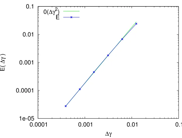
3.5.1. Convergence of the numerical scheme for the linear transport
We first study the convergence of the numerical scheme when the initial condition is centered in theSMphase C= (0.7,0.15) and the final time is small enough for the density to remain in this phase. The maturity function (3) and the source term (4) are both null, and the ageing function (2) is constant and equal to one. For such a constant linear transport, we can compute the exact solution at the final timetNt =t
maxusing the characteristic
method as well as the error inL1-norm of the numerical solution
E(∆γ) = ∆γ2
Nγ−1 X
k=0 Nγ−1
X
l=0 φ
Nt
k,l−φ0(ak+1 2 −t
Nt, γ l+1
2)
.
0.9 0.91 0.92 0.93 0.94 0.95 0.96 0.97 0.98 0.99 1
0 0.2 0.4 0.6 0.8 1 1.2 1.4 1.6
U(t)
t
a) Plasma FSH level
0.073 0.074 0.075 0.076 0.077 0.078 0.079 0.08 0.081 0.082 0.083
0 0.2 0.4 0.6 0.8 1 1.2 1.4 1.6
uf (t) t g2 g2 g2 g2 g2 g2 g2 g2 g2 g2 g2 g2 g2 g2 g2 g2 g2 g2 g2 0.50 0.55 0.60 0.65 0.70 0.75 0.80 0.85 0.90 0.95
b) Locally bioavailable FSH level
0.5 1 1.5 2 2.5 3
0 0.2 0.4 0.6 0.8 1 1.2 1.4 1.6
m0 (f,t) t g2 0.50 0.55 0.60 0.65 0.70 0.75 0.80 0.85 0.90 0.95
c) Cell mass of each follicle
1.5 2 2.5 3 3.5 4 4.5 5 5.5 6
0 0.2 0.4 0.6 0.8 1 1.2 1.4 1.6
M(t)
t
M(t)
Mo
d) Ovarian maturity
0.1 0.2 0.3 0.4 0.5 0.6 0.7 0.8 0.9 1
0 0.2 0.4 0.6 0.8 1 1.2 1.4 1.6
m(f,t) t g2 g2 g2 g2 g2 g2 g2 g2 g2 g2 g2 g2 g2 g2 g2 0.50 0.55 0.60 0.65 0.70 0.75 0.80 0.85 0.90 0.95 Mf
e) Maturity of each follicle
Figure 6. Competition between ten follicles differing by their ageing function parameterg2
1e-05 0.0001 0.001 0.01 0.1
0.0001 0.001 0.01 0.1
E(
∆γ
)
∆γ
0(∆γ2)
E
Figure 7. Convergence rate in the SM phase. Green curve : ∆γ→O(∆γ2). Blue curve : L1 norm error between the exact solution and the solution with space step∆γ.
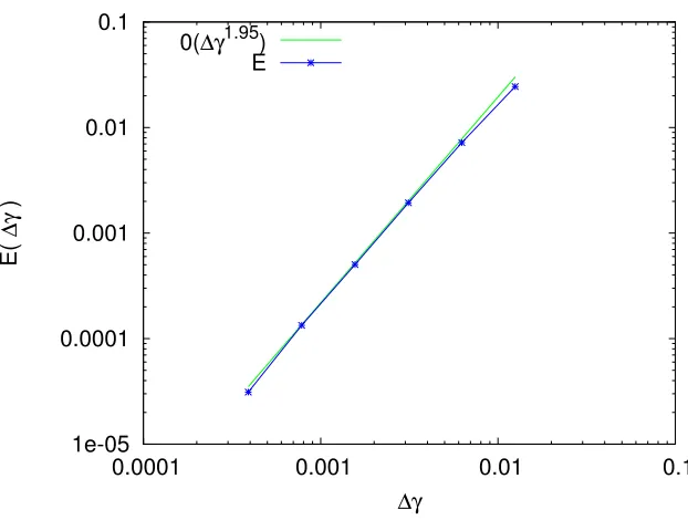
3.5.2. Full model convergence test
We now set the initial condition near the center C = (0.2,0.15) of the G1 phase, still with a maximum time tmax= 0.05 ensuring that the cell density remains in this zone. In that case the source term (4) and the age
and maturity speeds are no more constant, and we no longer know the exact solution of the PDE. The error is computed using the solution withNγ = 5120 as reference solution, that is compared to the solution on the
other meshes. Since we have used a dyadic refinement, the sizeNref of the reference mesh in one direction is
always a power of two times the sizeN∆γ of the current mesh. Denoting by P =
Nref
N∆γ
the ratio between the
current discretization and the reference finest one, we estimate the discretization error by
E(∆γ) = ∆γ2
N∆γ−1 X
k=0
N∆γ−1 X
l=0
φNt k,l−
1 P2
P X
p=0 P X
m=0
φrefkP+p,lP+m
The asymptotic orderO(∆γ1.95) which best fits the behavior ofE(∆γ) is displayed in Figure 8.
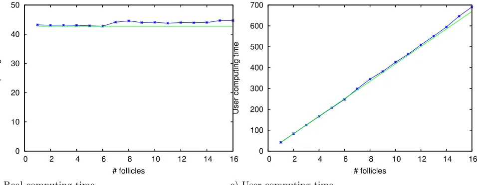
3.6.
HPC test
The improvement in terms of computing time provided by the parallelization is tested through a set of simula-tions involving an increasing number of identical follicles. The grid for these simulasimula-tions consists in one cycle of 200×200 cells, and the simulation goes on for 900 times steps. In this experiment, we disposed of enough processors to do the computing with one follicle by processor and since the timecommand is used to monitor the computing time, the output of the program has been commented out. Figure 9 a) shows the real computing time, which is basically the time elapsed from the beginning of the computation. Figure 9 b) shows the user computing time, which cumulates all the processors computing time. The computing time cannot be shorter than that required for a computation involving only one, this constitutes the so-called theoretical limit. The fact
1e-05 0.0001 0.001 0.01 0.1
0.0001 0.001 0.01 0.1
E(
∆γ
)
∆γ 0(∆γ1.95)
E
Figure 8. CV rate on the G1 phase. Green curve : ∆γ→O(∆γ1.95). Blue curve : L1 norm error between the reference solution and the solution with a space step ∆γ.
that the real computing time remains close to the computing time for one follicle and that the user computing time grows linearly with the number of follicles is very encouraging. The communications between processors appear not to affect significantly the gain in computing time due to the parallel computing. A small increase in real computing time can be noticed beyond eight follicles. This is due to the super calculator architecture, where the processors are pooled in eight processor nodes. The communications within one node are faster than across different nodes. This leads to a threshold effect observed as soon as more than eight processors are needed, therefore involving more than one single node.
Conclusion
This paper summarizes preliminary works in the development of a dedicated software to illustrate numerically the development of follicles. The uniform grid numerical method have been successfully tested in terms of robustness, accuracy and scalability on parallel architecture. As part of a challenging project involving biologists mathematicians and computer scientists, the different situations engendered by the model (mono-ovulation, poly-ovulation or anovulation) from given combinations of parameters will now be systematically and intensively tested. In order to achieve this goal within realistic delay the HPC aspect of the method must be enriched using adaptive mesh refinement. The multiresolution method developed in [5] and further tested and extended in [6] or [11] is currently implemented in this new configuration, where the presence of source terms and integral terms will require special considerations as exemplified for instance in [2].
Acknowledgment
The authors would like to thanks0 10 20 30 40 50
0 2 4 6 8 10 12 14 16
Real computing time
# follicles
a) Real computing time
0 100 200 300 400 500 600 700
0 2 4 6 8 10 12 14 16
User computing time
# follicles
c) User computing time
Figure 9. Parallelization performance test. Simulation of an increasing number of identical follicles. One follicle per processor. Green curve : theoretical limit. Blue curve : computing time (in seconds). Left : elapsed time from the start of the computation. Right : cumulative computed time on all processors
• Pascal Joly, Philippe Parnaudeau and Kyrill Pichon Gostaff3for their help concerning parallel comput-ing,
• the CIRM4for the excellent working conditions,
• the INRIA Large Scale Initiative Action REGATE5for the funding of the project.
References
[1] F. Bouchut and F. James. One-dimensional transport equations with discontinuous coefficients.Nonlinear Anal., 32(7):891–933, 1998.
[2] G. Chiavassa, R. Donat, and A. Martinez-Gavara. Cost-effective multiresolutions schemes for shock computations. In Mul-tiresolution and adaptive methods for convection-dominated problems, volume 29 ofESAIM Proc., pages 8–27. EDP Sci., Les Ulis, 2009.
[3] F. Cl´ement. Multiscale modelling of endocrine systems: new insight on the gonadotrope axis.ESAIM: Proc., 27:209–226, 2009. [4] F. Cl´ement, J.-M. Coron, and P. Shang. Optimal control for multiscale conservation laws describing the development of ovarian
follicles. 2011.
[5] A. Cohen, S. M. Kaber, S. M¨uller, and M. Postel. Fully adaptive multiresolution finite volume schemes for conservation laws.
Math. Comp., 72(241):183–225 (electronic), 2003.
[6] F. Coquel, Q. L. Nguyen, M. Postel, and Q. H. Tran. Entropy-satisfying relaxation method with large time-steps for Euler IBVPs.Math. Comp., 79(271):1493–1533, 2010.
[7] N. Echenim.Mod´elisation et contrˆole multi-´echelles du processus de s´election des follicules ovulatoires. PhD thesis, Universit´e Paris-Sud XI, Facult´e des Sciences d’Orsay, 2006.
[8] N. Echenim, F. Cl´ement, and M. Sorine. Multiscale modeling of follicular ovulation as a reachability problem. Multiscale Model. Simul., 6(3):895–912, 2007.
[9] N. Echenim, D. Monniaux, M. Sorine, and F. Cl´ement. Multi-scale modeling of the follicle selection process in the ovary.Math. Biosci., 198(1):57–79, 2005.
[10] E. Godlewski and P.-A. Raviart. The numerical interface coupling of nonlinear hyperbolic systems of conservation laws. I. The scalar case.Numer. Math., 97(1):81–130, 2004.
3Laboratoire Jacques-Louis Lions, UPMC-Paris 6 4http://www.cirm.univ-mrs.fr
5https://www.rocq.inria.fr/sisyphe/reglo/regate.html
[11] N. Hovhannisyan and S. M¨uller. On the stability of fully adaptive multiscale schemes for conservation laws using approximate flux and source reconstruction strategies.IMA J. Numer. Anal., 30(4):1256–1295, 2010.
[12] R.J. LeVeque. Wave propagation algorithms for multidimensional hyperbolic systems.J. Comput. Phys., 131(2):327–353, 1997. [13] R.J. LeVeque and M.J. Berger. Adaptive mesh refinement using wave-propagation algorithms for hyperbolic systems.SIAM
J. Numer. Anal., 35(6):2298–2316, 1998.
[14] P. Michel. Multiscale modeling of follicular ovulation as a mass and maturity dynamical system. Multiscale Model. Simul., 9(1):282–313, 2011.
[15] P. Shang. Cauchy problem for multiscale conservation laws : Applications to structured cell populations. http://arxiv.org/abs/1010.2132, 2010.
[16] P. K. Sweby. High resolution schemes using flux limiters for hyperbolic conservation laws.SIAM J. Numer. Anal., 21(5):995– 1011, 1984.