A comparative study between kriging and adaptive sparse tensor-product methods for multi-dimensional approximation problems in aerodynamics design*

N. Champagnat, T. Leli`evre, A. Nouy, Editors

A COMPARATIVE STUDY BETWEEN KRIGING AND ADAPTIVE SPARSE

TENSOR-PRODUCT METHODS FOR MULTI-DIMENSIONAL

APPROXIMATION PROBLEMS IN AERODYNAMICS DESIGN

Abdellah Chkifa

, Albert Cohen

, Pierre-Yves Passaggia

and Jacques Peter

Abstract. The performances of two multivariate interpolation procedures are compared using func-tions that are either synthetic or coming from a shape optimization problem in aerodynamics. The aim is to evaluate the efficiency of adaptive sparse interpolation algorithms [2] and compare them with the kriging approach developed for the design and analysis of computer experiment (DACE) [21]. The accuracy and computational time of the two methods are examined as the numberN of samples used in the interpolation increases. It appears in our test cases that both methods perform equivalently, in terms of precision. However, as the dimensiondincreases, the computational time involved in the enrichement of the kriging sample becomes intractable for large values of N. This problem is cir-cumvented in the case of the sparse interpolation procedure for which the computational time scales linearly withN andd.

R´esum´e. Nous comparons les performances de deux m´ethodes d’interpolation en grande dimension, aussi bien sur des fonctions synth´etiques que pour celles issues d’un probl`eme d’optimisation de forme en aerodynamique. L’objectif est d’´evaluer l’efficacit´e d’algorithmes adaptatifs d’interpolation parci-monieuse [2], et de les comparer avec l’approche du kriging d´evelopp´ee dans le cadre design and analysis of computer experiment (DACE) [21]. La pr´ecision et le temps de calcul des deux m´ethodes sont ´etudi´es lorsque le nombreN d’´echantillons utilis´es pour l’interpolation augmente. Les cas tests montrent que les deux m´ethodes sont comparables en terme de pr´ecision. Cependant, lorsque la dimension d aug-mente, le temps de calcul associ´e `a l’enrichissement de l’´echantillon pour le kriging devient prohibitif pour les grandes valeurs deN. Ce probl`eme est contourn´e dans le cas de l’interpolation parcimonieuse pour lequel le temps de calcul est lin´eaire enN etd.

1.

Introduction

Surrogate models, such as the surface response method are becoming increasingly popular in performing various optimization or uncertainty quantification studies for parameter dependent complex problems. Such problems are difficult to handle numerically, especially in high dimension, that is, when the number d of parameters is large. Surrogate models are a non intrusive approach that aim at providing a simplified and computable representation of the solution in the parameter space. The principle of a surrogate model relies on an efficient interpolation procedure that estimates a scalar or vector field using a sampled data set. Each sample typically corresponds to an instance of the solution of a complex problem, often computationally expensive.

∗_{Acknowledgements: the authors thank ONERA, IUF and UPMC for their support during the CEMRACS of 2013.}

1 _{LJLL, Universit´e Pierre & Marie Curie, 75005, Paris, France} 2 _{Onera, The French Aerospace Lab. 92322 Chˆatillon, France}

©EDP Sciences, SMAI 2015

It is therefore mandatory that the procedure achieves the required accuracy for a reasonable number N of samples, and that the CPU time required for the construction of the interpolant remains negligible compared to that of the instances computation. Efficient algorithms are particularly needed as the number of variablesd

increases due to the so-called curse of dimensionality. In particular, one may significantly gain by considering adaptive strategies, for which every new sample is chosen based on the information gained through the previous interpolation procedure. Here, two such strategies are being considered.

● The kriging procedure, initially developed by [11] has become increasingly popular over the past decades, due to its robustness in the sense that the interpolation points may be at arbitrary locations. This approach assumes that the function to be interpolated, is the realization of a stochastic process and computes the interpolant at a given point as a best unbiased linear estimator from the available data set. The relation between the interpolation and the current sample is based on a covariance function, often assumed to be of gaussian form, with internal parameters that have to be optimized in order to provide a reliable estimate. In an adaptive context, the variance of this estimator also provides with a way to select the location for additional data to be included in the data sample, in order to improve the accuracy of the surrogate model.

● Sparse approximation methods, originally developed by [24] in the context of quadrature rules, also became popular over the past decades. These methods aim at constructing high precision polynomial or piece-wise polynomial approximations while retaining a limited number of grid points through the introduction of a specific sparse grid. In recent years, adaptive versions have been introduced and studied, in particular in [2] for the polynomial case based on a greedy strategy which selects the next sparse grid point in order to minimize the interpolation error.

Our present study is motivated by shape design problems in aerodynamics. For instance, minimizing drag at constant lift of an aerofoil, at cruise flight conditions, is of major importance since it results in substantial savings of fuel consumption. The basic idea is to prescribe control points around a two-dimensional aerofoil and alter the geometry using CAD functions such as B-spline functions for example [10, 12]. This topic has been treated extensively over the past decades [4, 7–9, 14, 17, 22]. However, most studies appeared to report up to 6 design parameters and less than 5000 samples for evaluating the surrogate model. Beyond this limit, the commonly used interpolation procedures appear to be far more computationally expensive than the aerodynamics code itself. For instance when considering the kriging procedure [12], the computational time evolves cubically with the number of evaluation points N. In addition, the optimization of the internal parameters of the problem requires minimizing a non-convex cost function defined on a space of dimension d, whered is the number of variables, the evaluation of which requires by itselfO(N3_{)operations. Therefore the total computational grows} fastly withN and this effect is even more accentuated in high dimension. Note in addition that the value ofN

needed to obtain a reliable estimate typically grows with d, due to the so-called curse of dimensionality. An alternative approach which aim to alleviate the curse of dimensionality is provided by the use ofsparse

grids. Sparse grid methods have been introduced by Smolyak in the context of numerical integration [24]. They

are based on particular unions of tensor product grids for which fineness in one variable is typically compensated by coarseness in other variables. This approach has been extensively applied to uncertainty quantification [29,30] and applied to aerodynamics recently, see [13, 28] for a review. Very recently, [19] have applied this method for the case of a subsonic aerofoil using 14 uncertain parameters. However there is a lack in the literature when considering surface response methods using sparse grid interpolation approaches. Moreover, surface response methods appear to be efficient methods on non-intrusive robust optimization problems where one has to optimize a design subject to uncertainty, see [5] for a recent review. Here, we want to investigate the already mentioned adaptive versions of sparse grid interpolation introduced in [2] in the polynomial case. We are also interested in adapting this approach to the piecewise polynomial case which is better adapted to the presence of locally sharp regions or discontinuities in the function to be interpolated.

The rest of the paper is organized as follow. We successively detail in§2 the kriging and sparse interpolation adaptive algorithms. For both methods, we discuss several adaptive strategies for the enrichment of the sampling set. We then present in §3 two test cases, namely a synthetic function and the lift to drag ratio of a two-dimensional aerofoil in a transonic flow as a function of shape parameters. These test cases reveal that both adaptive interpolation algorithms behave similar in terms of precision with respect to the numberN of samples. However, the adaptive kriging algorithm becomes computationally intractable for large values ofdandN, while the CPU cost of the sparse interpolation algorithm is linear in bothN andd. This advocates for the use of this second class of algorithms for high-dimensional problems. Some conclusions and perspectives are drawn in §4.

2.

Methods

In the present investigation, the aim is either to approximate or optimize a function

y↦f(y), (1)

where the coordinate vector y = (y1, . . . , yd) concatenates the various parameters of a given model problem, and f(y) ∈R is a quantity of interest computed from the solution of this problem for the particular value of

y. For simplicity we assume thaty ranges in the hypercubeU = [−1,1]d. There is no loss of generality in this assumption when everyyj ranges independently in a finite intervalIj since we may then use a standard affine change of variable betweenIj and[−1,1].

The objective is to build an accurate numerical approximation off or ofM ∶=maxy∈Uf(y)using the smallest possible numberN of evaluationsf(yi_{)at given pointsy}i_{∈U from a sampling setS}

N = {y1, . . . , yN}. Of course, if an approximation ˜f tof has been computed, one way of approximatingM is byM∶=maxy∈Uf˜(y). However the specific search for the maximum may benefit from using different sampling setsSN for a givenN than when searching for a global approximation tof.

2.1.

The kriging procedure

Kriging is based on the hypothesis [15] that the unknown functionf is random can be decomposed into

f(y) =µ(y) +g(y), (2)

where µ(y)and g(y)are sought as a deterministic contribution from a low-dimensional space and a random fluctuation respectively. Typically, we search forµas a constant or low order polynomial. The random process

g is assumed to be centered, second order, with covariance kernel of stationary form

Cov(g(y), g(z)) =E(g(y)g(z)) =φ(y, z) =ϕ(y−z). (3)

In this framework, the kriging interpolation tof(y)is a linear combination

INf(y) ∶= N ∑ i=1

λi(y)f(yi), (4)

defined as the best linear unbiased estimator, in the sense that it minimizes the mean square error

E(∣f(y) − N ∑ i₌1

λif(yi)∣2), (5)

over all choices of λi _{under the constraint that}

E(∑Nn=1λif(yi)) =E(f(y)). This minimization problem leads

● Ordinary kriging: µis constant and unknown.

● Universal kriging;µis an unknown polynomial of known order.

The ordinary kriging is by far the most popular approach and we use it in the present investigation. In this case, the unbiased constraint implies that ∑Ni₌1λi(y) =1, which also means that the interpolation process is exact for constants. Denoting byχ the Lagrange multiplier, the resulting linear system for finding theλi(y)is given by ⎡⎢ ⎢⎢ ⎢⎢ ⎢⎢ ⎣

φ(y1, y1) ⋯ φ(y1, yN) 1

⋮ ⋱ ⋮ 1

φ(yN_{, y}1_{) ⋯ φ(y}N_{, y}N_{) 1}

1 ⋯ 1 0

⎤⎥ ⎥⎥ ⎥⎥ ⎥⎥ ⎦ ⎡⎢ ⎢⎢ ⎢⎢ ⎢⎢ ⎣ λ1 ⋮ λN χ ⎤⎥ ⎥⎥ ⎥⎥ ⎥⎥ ⎦ = ⎡⎢ ⎢⎢ ⎢⎢ ⎢⎢ ⎣

φ(y1, y)

⋮

φ(yN, y)

1 ⎤⎥ ⎥⎥ ⎥⎥ ⎥⎥ ⎦ . (6)

Standard linear algebra manipulations show that the resulting interpolant also writes

INf(y) = N ∑ i=1

βiφ(yi, y) +βN+1, (7)

where the weightsβi are solution to the system

⎡⎢ ⎢⎢ ⎢⎢ ⎢⎢ ⎣

φ(y1_{, y}1_{) ⋯ φ(y}1_{, y}N_{) 1}

⋮ ⋱ ⋮ 1

φ(yN_{, y}1_{) ⋯ φ(y}N_{, y}N_{) 1}

1 ⋯ 1 0

⎤⎥ ⎥⎥ ⎥⎥ ⎥⎥ ⎦ ⎡⎢ ⎢⎢ ⎢⎢ ⎢⎢ ⎣ β1 ⋮ βN

βN₊1 ⎤⎥ ⎥⎥ ⎥⎥ ⎥⎥ ⎦ = ⎡⎢ ⎢⎢ ⎢⎢ ⎢⎢ ⎣

f(y1)

⋮

f(yN₎ 0 ⎤⎥ ⎥⎥ ⎥⎥ ⎥⎥ ⎦ , (8)

The expression of the kriging interpolant by (7) is therefore more convenient since the system to be solved does not depend on y. It reveals that the interpolant is a linear combination of the constant function and of the functions y↦φ(yi, y)fori=1, . . . , N.

The covariance kernel φ(y, z) has to be positive definite. A frequently considered form, that we use in the present investigations, is the gaussian

φ(y, z) =exp{ −1 2

d ∑ k₌1

(yk−zk)2

ζ2 k

}. (9)

The kernel parameters (ζ1, . . . , ζd) could be fixed a-priori, however in order to improve the accuracy of the interpolation process they should rather be adjusted with the objective of minimizing the error between f(y)

and its interpolation INf(y). Here, we use a standard cross validation procedure, the so-called leave-one-out method, that consists in removing a pointyi from the sampling set SN and computing the error between the kriging interpolantIi

N−1f(y

i_{)computed fromS}

N−{yj}and the exact valuef(yi). We then selectζ= (ζ1, . . . , ζd) by minimizing the mean square error

E(ζ) = 1 N

N ∑ i=1

(f(yi) −I_Ni ₋₁f(yi))2. (10)

The computations of theN interpolantsI_Ni₋₁f can be done efficiently using Rippa’s method [20]. However, the optimization task becomes computationally intensive asdand/orN become moderately large, even when using the algorithm proposed in [26].

One typical predefined sampling set, that we consider in the present investigations, is given by the section

SN = {y1, . . . , yN} from the Halton sequence

yn=⎡⎢⎢⎢

⎢⎢ ⎣

2γq1(n) −1 ⋮ 2γqd(n) −1

⎤⎥ ⎥⎥ ⎥⎥ ⎦

, (11)

whereq1,⋯, qdare the firstdprime numbers, and whereγq(n) =n0q−1+n1q−2+ ⋯ +nmq−m−1withnpsuch that

n=n0+n1q+n1q2+ ⋯ +nmqmin the q-adic expansion (see for instance [18]). This sequence aims at building for eachN a quasi-uniform sampling set overU.

Adaptive strategies for building the sampling set are based on the mean square error function

y↦σ2(y) ∶=_E(∣f(y) −INf(y)∣2) (12)

which can be explicitely computed at each y for the kriging estimator. One first strategy consists in selecting the new pointyN+1 which maximizesσ2(y)overU. In contrast to the Halton sequence, this strategy may lead to non-uniform distributions in the sampling sets. In particular, more data points are likely to be introduced in the directions where the covariance parametersζk are small.

In our numerical tests, we perform the search for the new pointyN+1 based on maximizingσ(y) using the same differential evolution algorithm as used for the optimization of the correlation vectorζ. The computation cost of both optimization procedures constitute a significant computational bottleneck for the adaptive kriging algorithm asdandNboth get large. In addition, the computation of the kriging approximation requires solving a N×N system with a full matrix, typically amounting inO(N3_)complexity.

2.2.

The sparse interpolation procedure

The sparse interpolation procedure in arbitrary dimension is based on tensorization-sparsification of a hierar-chical interpolation procedure in one dimension. We recall in a nutshell the idea for polynomial interpolation as proposed and analyzed in [2], then show how the procedure can be generalised to other types of interpolation.

Given the dimensiond, the multivariate polynomial spaces considered are of the general form

PΛ∶=Span{yν =yν11. . . y νd

d ∶ ν= (ν1, . . . , νd) ∈Λ}, (13)

where Λ∈Nd is an index set that is assumed to be downward closed (also called lower set), in the sense that,

givenν, µ∈Nd,

ν∈Λ and µi≤νi, i=1, . . . , d ⇒ µ∈Λ. (14)

Consider any infinite sequence Z ∶= (zi)i_≥0 of pairwise distinct points in [−1,1], and denote by Ik the univariate Lagrange interpolation operator onto Pk associated with the section{z0,⋯, zk}. The operators Ik can be computed recursively. Indeed, for anyk≥0, the difference operator ∆k∶=Ik−Ik₋1 can be expressed as

∆kf= (f(zk) −Ik−1f(zk))hk, h0(z) =1, hk(z) = k−1 ∏ j=0

z−zj

zk−zj

, (15)

with the convention I₋1 is the null operator. Now, for an arbitrary lower set Λ⊂Nd, we introduce the grid of

points

ΓΛ∶= {zν∶ν∈Λ} where zν∶= (zνj)j=1,...,d∈ [−1,1]

d

. (16)

It is proved in [2] that the grid ΓΛis unisolvant for the polynomial spacePΛand that the interpolation operator is given by

IΛ∶= ∑ ν∈Λ

We observe that this coincides with the telescopic sumIk= ∑kj=0∆k for the univariate cased=1. Similarly to the univariate case, it has been proved in [2] that the hierarchical computation of the interpolation operatorIΛ is possible. More precisely, given a lower set Λ and any multi-indexν ∈Nd∖Λ such that Λ′∶=Λ∪ {ν}is a lower

set, the operatorIΛ′ is the sum ofI_Λ and the increment operator ∆_ν which can be computed using

∆ν= (f(zν) −IΛf(zν))Hν, Hν∶= ⊗dj₌1hνj. (18)

The stability of the operatorsIΛis critical for numerical applications, such as the design of surrogate models from computer experiments. It is measured by the Lebesgue constant

LΛ∶= max f_∈C₍U_)−{0_}

∥IΛf∥L∞(_U) ∥f∥L∞(_U)

. (19)

This constant depends on the sequence Z, in particular through the Lebesgue constants Lk of the univariate interpolation operators Ik defined similarly. It was shown in [2] that algebraic growth of Lk yields algebraic growth of the Lebesgue constantLΛ. More precisely

Lk≤ (1+k)θ, for any k≥1 Ô⇒ LΛ≤ (#Λ)θ+1. (20)

Surprisingly, the previous implication is valid whatever the dimension dand the shape of the finite lower set Λ. We note that sequences Z with provable slow algebraic growth of the Lebesgue constant _Lk exist in the literature. These sequences are known as R-Leja sequences [1]. They can be computed explicitely and we use them in our numerical tests for sparse polynomial interpolation.

The tensorization-sparsification approach used in the construction of the polynomial interpolation procedure can be generalized to other types of interpolation. We describe the approach in an abstract context. We consider the following sets

(T,≤), Z_T ∶= {zλ ∶ λ∈ T }, HT ∶= {hλ ∶ λ∈ T }, (21) that stands respectively for a countable partially ordered set of indices, a sequence indexed in T of pairwise distinct abscissas in[−1,1]and a hierarchical basis indexed inT of functions onC([−1,1])satisfying

hλ(zλ′) =δ_λ,λ′, if λ′≤λ. (22)

We consider the set of multi-indices Td∶= {ν= (ν1, . . . , νd) ∶νj ∈ T } and define lower sets Λ⊂ Td similarly to (14) with≤being the partial order overT. For a lower set Λ, we introduce

ΓΛ∶= {zν∶= (zν1, . . . , zνd) ∶ν∈Λ}, HΛ∶=span{Hν∶= ⊗

d

j=1hνj ∶ν∈Λ}, (23)

the grid of interpolation points and the space of interpolation. The same arguments as used in [2] for the polynomial setting show that the grid ΓΛ is unisolvant for the space HΛ. In the general context where T might not be totally ordered, the formula (17) does not make clear sense, yet we may still rely on the recursive computation of the interpolation operators. Namely, if Λ is lower set andν∈ Td∖Λ such that Λ′=Λ∪ {ν} is a lower set, then we have

IΛ′f =I_Λf+ (f(z_ν) −I_Λf(z_ν))H_ν. (24)

For numerical experiment, we consider dyadic hierarchical piecewise linear or piecewise quadratic interpola-tion. For such interpolation procedures, the set T is defined by

induced with the partial orderλ₋1≤λ1≤ (0,0)and

(j, k) ≤ (j+1,2k), (j, k) ≤ (j+1,2k+1), (j, k) ∈ T. (26)

The setT is a binary tree whereλ₋1is the root node,(0,0)is a child ofλ1which is a child ofλ−1, every node (j, k)has two children (j+1,2k) and (j+1,2k+1), and the relation λ′≤ λ meansλ′ is a parent ofλ. We associate withT the set of abscissas

Z_T ∶= {zλ−1, zλ1, z(0,0)} ∪ {z(j,k)∶= 2k+1

2j ∶ (j, k) ∈ T, j≥1}, (27)

where zλ−1 = −1, zλ1 = 1 and z(0,0) = 0. We also associate with T the hierarchical basis of piecewise linear functions H_T = {hλ∶λ∈ T }defined over[−1,1]by

hλ−1(s) =1, hλ1(s) =

1+s

2 , h(j,k)(x) =ψ(2 j₍

s−zj,k)), ψ(s) ∶=max{0,1− ∣s∣}, (j, k) ∈ T, (28)

It is easy to verify that the functionhλand the abscissaszλsatisfies the condition (22), therefore the hierarchical interpolation can be performed. Let us note that in dimensiond=1, the hierarchical interpolation amounts in first approximatingf by the constant function of valuef(−1), second by the affine function that coincides with

f at−1 and 1, third by the piecewise affine function that coincides withf at−1, 0 and−1, and in further steps refine by interpolating at the midpoint of an interval between two adjacents interpolation points. The indexj

corresponds to the level of refinement, or the depth of the node in the binary tree.

In the case of piecewise quadratic interpolation, the procedure is exactly the same, except that the hierarchical basis is nows given by

hλ−1(s) =1, hλ1(s) = ( 1+s)2

4 , h(j,k)(x) =ψ(2 j₍

s−zj,k)), ψ(s) ∶=max{0,1−s2}, (j, k) ∈ T. (29)

which corresponds to interpolation by piecewise quadratic functions with the same ordering on the interpolation points as in the piecewise affine case.

Having fixed the sparse interpolation procedure (polynomial, piecewise affine or piecewise quadratic), the problem is now to select lower sets Λ giving the best possible interpolation spacesHΛ (orPΛin the polynomial case) for the target functionf. In the non-intrusive context that motivated this work, no prior information is known onf, whence the optimal approximation space _HΛ for a givenN =#(Λ)is not accessible. Therefore, we may only rely on greedy type strategies. The recursive formula (24) suggests to couple the interpolation algorithm with an adaptive strategy for the choice of best multi-index ν used to enrich Λ. Given Λ a lower set, we denote N (Λ)the set of adjacent neighbours to Λ, which are the multi-indices ν ∈ Td_{∖Λ such that} Λ′∶=Λ∪ {ν}is a lower set. Depending on the approximation context, we choose to enrich Λ byν∈ N (Λ)that either satisfies

● the supremum norm of the increment∥∆νf∥L∞(_U) is maximal, ● the least square norm of the increment∥∆νf∥L2_(U)is maximal, ● the valuef(zν)is maximal.

The two first criterions are designed for the approximation off in theL∞ and theL2 _{sense, respectively, while} the third criterion is designed for optimization and can be seen as a way of exploring the local maxima off.

Although the set of candidates N (Λ) might be very large, the enrichment step requires at most d new evaluations off. Indeed, forν∈Λ and Λ′=Λ∪ {ν}, the setN (Λ′) ∖ N (Λ)contains at mostdindices. We also note that for the two first strategies, the computation of∥∆νf∥for the new indices consists merely in computing

∣f(zν) −IΛf(zν)∣ d ∏ j=0

with∥⋅∥being theL∞or theL2_{norm. This is computationally fast since theh}

nare known in advance and their norm∥hn∥can be tabulated. The cost of the computation∥∆νf∥is essentially dominated by the evaluation of

f(zν)in cases wheref is evaluated through a heavy numerical solver.

While the above strategies often give good numerical results in practice, they can be defeated when the target function has oscillations that fail to be captured by the greedy selection procedure. For example, consider the two first criterions for piecewise linear adaptive interpolation of a univariate function f such that f(1₂) =

1

2(f(0)+f(1)). Then, the increment corresponding to the pointz(1,0)= 12 is ∆(1,1)f =0. Therefore the adaptive algorithm might fail to explore the region[0,1]on whichf could still oscillate away from its linear interpolation. Similarly an algorithm based on the third criterion could be trapped in local maximas.

One way to remedy this defect consists in modifying the algorithm a follows: we produce the nested sequence of lower sets

Λ1⊂Λ2⊂ ⋯ ⊂ΛN ⊂ ⋯

with #(ΛN) = −N, by alternatingp−1 adaptive steps where the new indexν∈ N (ΛN)is picked based on the chosen criterion whenN∉pN, and one “conservative” step where we pick the most “ancient” indexν∈ N (ΛN) when N∈pN, in the sense that it has been lying inN (Λk)for the smallest value of k≤N. This conservative step allows us to explore the whole parameter spaceU, while retaining the adaptive feature of the algorithm. In our numerical test we have used the valuep=5, based on empirical observation that it gives a good balance between adaptivity and exploration.

An important feature of these adaptive algorithm is that the computational cost scales like d+N, where

N =#(ΛN) and d is the dimension. Indeed, the construction of ΛN+1 from ΛN requires inspecting at most

d new values of the unknown function. This contrasts with the kriging algorithm and will be reflected in the numerical tests.

3.

Numerical tests

3.1.

Synthetic functions

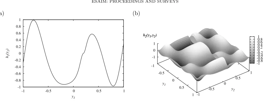
The performances of the above algorithms have been assessed on two classes of problems. First, two synthetic functions are considered. The first is a smooth one-dimensional sinusoidal type function whereas the second is two-dimensional and exhibits a sharp gradient along one abscissa, depicted in figure 1. The synthetic functions are given by

h1(y1) ∶=g(10y1−2)cos(y21); g(s) ∶=

s∣s∣

1+s2, (31a)

h2(y1, y2) ∶=g(10y1−2)cos(5y1)2 g(100y2−20)cos(5y22). (31b)

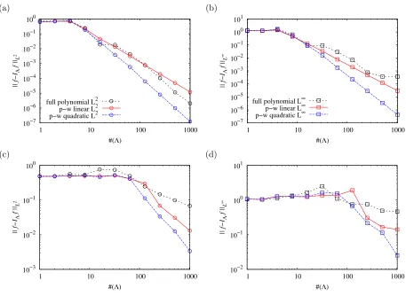
These functions are evaluated in the domain U = [−1,1]d _{with d = 1 and 2 respectively, and displayed on} Figure 1. The univariate functionh1 is smooth with a kink aty1=0.2. The two-dimensional function h2 has a sharp gradient along y2 =0.2. The sparse interpolation algorithm is first considered and the performances are compared on Figure 2 between the polynomial, piecewise linear and piecewise quadratic procedures. The

L∞ and L2 errors in all figures have been computed based on 106 randomly chosen samples. For the two test cases, the piecewise quadratic algorithm shows the best convergence. This procedure is higher accurate than its piecewise linear counterpart, while still providing local adaptivity as opposed to its polynomial counterpart. A comparison with the kriging procedure is shown on Figures 3 where results between the piecewise quadratic sparse interpolation appears to be more precise than the kriging using the Halton sequence.

(a)

-1 -0.8 -0.6 -0.4 -0.2 0 0.2 0.4 0.6 0.8 1

-1 -0.5 0 0.5 1

h1 (y1

)

y₁

(b)

-1

-0.5

0

0.5

1 -1 -0.5

0 0.5

1 -1

0 1 h2(y1,y2)

y1

y2 h2(y1,y2)

-1 -0.8 -0.6 -0.4 -0.2 0 0.2 0.4 0.6 0.8 1

Figure 1. Sketch of the one-dimensional (a) and two-dimensional (b) synthetic functions, given in equations (31a) and (31b)

procedure, we have observed that the selected interpolation points are mainly clustered along the sharp gradient region. In the case of the Kriging, the internal parameterζ2appears to be much smaller thanζ1, and the points appear to be mostly distributed along the y2 direction. Note that due to the computational time involved in computing the adaptive kriging, the results for #(Λ) >512 could not be computed as the parameters for the kriging are recomputed every time a new point is included in the data set. We discuss later the comparison between computational costs.

3.2.

Surrogate model for a transonic wing profile

The second class of problem studied is a transonic flow over a RAE2822 wing profile. The flow solution is computed using the MISES code [6] which solves the Euler equations together with a boundary layer correction. Results are shown on Figure 4 for the baseline solution, compared with the data from the experiment in [3] for similar inflow conditions. The inflow conditions are given by the Mach number M = 0.729, the angle of attackα=2.31o _{and the Reynolds numberRe=10}6 _{based on the chord lengthc and the flow at infinity. The} pressure distribution, shown on Figure 4(a) exhibits a discontinuity on the suction side of the aerofoil, denoting the presence of a shock, caused by the expanding geometry of the aerofoil after c>0.4. In the present study, the value of interest is given by the ratio between the lift and the drag

f= Cl Cd

(32)

where

Cl= ∫ ξ

p(s)nα(s)ds, and Cd= ∫ ξ

p(s)tα(x)ds, (33)

where nα = n⋅ (−_cossin₍(_αα₎)) and tα = n⋅ (cos_sin((_αα)₎) with n the outward normal vector. The shape of the baseline RAE2822 profile has been altered using four B-spline functions. More precisely

● The 4 control points are located at 5,20,40 and 60% of the chordc, see Figure 4(a).

● The amplitude of each B-spline is taken in the interval [−1.7510−3_c,1.7510−3_{c]and is directed towards} the normal to the initial profileξ.

● The leading edge and the trailing egde have been considered as fixed.

(a)

10−7 10−6 10−5 10−4 10−3 10−2 10−1 100

1 10 100 1000

|| f−I

Λ

f ||

L

2

#(Λ) full polynomial L2

p−w linear L2 p−w quadratic L2

(b)

10−7 10−6 10−5 10−4 10−3 10−2 10−1 100 101

1 10 100 1000

|| f−I

Λ

f ||

L

∞

#(Λ) full polynomial L∞

p−w linear L∞ p−w quadratic L∞

(c)

10−3

10−2

10−1

100

1 10 100 1000

|| f−I

Λ

f ||

L

2

#(Λ)

(d)

10−2 10−1 100 101

1 10 100 1000

|| f−I

Λ

f ||

L

∞

#(Λ)

Figure 2. Comparison between the polyomial, piecewise linear and piecewise quadratic sparse adaptive interpolation procedures: L2 _{error (left), L}∞ _{error (right), function h}

1 (up) and functionh2 (down).

pressure gradient induced by the geometry of the profile. Even for small variations of the shape parameterw, the pressure gradient is altered significantly, which leads to nonlinear variations of the lift and the drag.

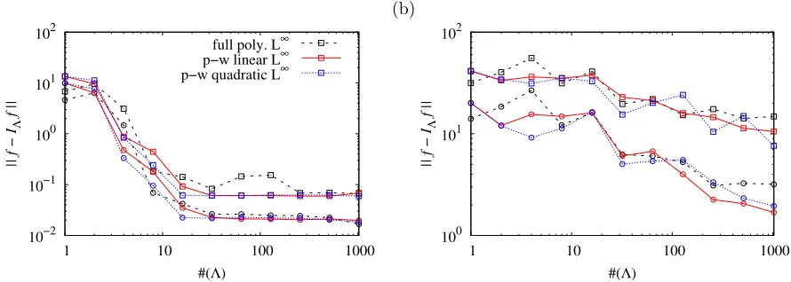
The kriging and the sparse adaptive algorithm are compared for different sample size and in several dimen-sions. The three procedures for sparse interpolation are compared on Figures 5. Similar to the synthetic case, the polynomial procedure is the least accurate whereas the piecewise linear and piecewise quadratic procedures appear to perform equally for both theL2 andL∞error. The two kriging procedure (Halton and adaptive) are then compared on figure 6. The results appear to be comparable for sampling sizes #(Λ) ≤128. Beyond this limit, the adaptive kriging appears to perform slightly better for theL∞error. We observed that the valued of the internal parameters ζ are fairly similar and that the points selected by the adaptive procedure tend to be more clustered along the borders. This is due to the fact that the kriging suffers from the lack of data points beyond the limit of the parameter space and thus tends to cluster extra points on the boundaries.

(a) 10−7 10−6 10−5 10−4 10−3 10−2 10−1 100

1 10 100 1000

|| f − I

Λ

f ||

L

2

#(Λ)

p−w quad. L∞ krig. Halton krig. adapt. (b) 10−7 10−6 10−5 10−4 10−3 10−2 10−1 100 101

1 10 100 1000

|| f − I

Λ

f ||

L

∞

#(Λ)

(c)

10-3 10-2 10-1 100

1 10 100 1000

|| f - I

Λ

f ||

L

2

#(Λ)

(d)

10-2 10-1 100 101

1 10 100 1000

|| f - I

Λ

f ||

L

∞

#(Λ)

Figure 3. Comparison between the Kriging using either the Halton sequence or the adaptively selected sequence, and the piecewise quadratic sparse adaptive interpolation: L2 _{error (left),}

L∞ error (right), functionh1(up) and functionh2(down).

(a) -2 -1.5 -1 -0.5 0 0.5 1 1.5

0 0.2 0.4 0.6 0.8 1

ξ p( ξ ) c (b) -0.0015 -0.001 -0.0005 0 0.0005 0.001 0.0015

y1 _-0.0005-0.001-0.0015

0 0.0005 0.001

0.0015 y2

40 50 60 70 80 90 f(y₁,y₂,0,0)

40 45 50 55 60 65 70 75 80 85

(a)

10−2

10−1

100

101

102

1 10 100 1000

|| f − I

Λ

f ||

#(Λ)

full poly. L∞

p−w linear L∞

p−w quadratic L∞

(b)

100

101

102

1 10 100 1000

|| f − I

Λ

f ||

#(Λ)

Figure 5. Comparison of the L∞ (◻) and the L2 error (_#) for the sparse interpolation al-gorithms applied to the functions y1 ↦f(y1,0,0,0)(a) and (y1, y2, y3, y4) ↦f(y1, y2, y3, y4) (b).

(a)

10−2 10−1 100 101

1 10 100 1000

|| f − I

N

f ||

#(Λ)

krig adapt. krig. Halton

(b)

10−1 100 101 102

1 10 100 1000

|| f − I

N

f ||

#(Λ)

Figure 6. Comparison of theL∞(∎) and theL2error ( ) for the kriging algorithms applied to the functionsy1↦f(y1,0,0,0)(a) and(y1, y2, y3, y4) ↦f(y1, y2, y3, y4)(b).

in the introduction of this paper, and are related in particular to theO(N3_{)complexity of the inversion process} in the kriging procedure.

4.

Conclusions

(a)

10−2

10−1

100

101

102

1 10 100 1000

|| f − I f ||

#(Λ)

p−w linear L∞

adapt. krig.

(b)

10−1 100 101 102

1 10 100 1000

|| f(y) − I f(y) ||

#(Λ)

Figure 7. Comparison of theL∞error (◻piecewise linear sparse,∎adaptive kriging) and of theL2_{error (}

#piecewise linear sparse, adaptive kriging), for the functionsy1↦f(y1,0,0,0) (a) and(y1, y2, y3, y4) ↦f(y1, y2, y3, y4)(b).

10−3

10−2

10−1

100

101

102

103

104

105

106

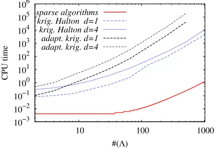
10 100 1000

CPU time

#(Λ)

sparse algorithms krig. Halton d=1 krig. Halton d=4 adapt. krig. d=1 adapt. krig. d=4

Figure 8. Comparison of the CPU time between adaptive and non-adaptive kriging ford=1 andd=4 and adaptive sparse interpolation ford=4.

recently devoted to the kriging procedure, it appears that beyond a sampling #(Λ)of a few hundred points, the surrogate model to compute becomes expensive. Beyond a few thousand samples, the kriging surrogates might become more computationally expensive to evaluate than the CFD solver itself, which questions the relevance of this surrogate model for large scale engineering applications. This comparison between kriging and adaptive sparse interpolation has been carried out for fairly low-dimensional problems (up tod=4) when compared with full size engineering applications. However, these results clearly show that both methods provide comparable accuracy but at significantly different computational cost, which clearly advocates in favour of the sparse adaptive interpolation procedure for computing surrogate models.

Acknowledgements

P.-Y. Passaggia acknowledges the support by the French ”Agence Nationale pour la Recherche” (ANR

References

[1] Chkifa, A. On the Lebesgue constant of Leja points on the unit disk and their real projectionsJ. Approx. Theory, 166 :176-200, 2013 .

[2] Chkifa, A. and Cohen, A., Schwab, C., High-dimensional adaptive sparse polynomial interpolation and applications to para-metric PDEs.Research Report ETHZ, No 2012-22, 2012.

[3] Cook, P. H., and M. A., McDonald and, Firmin., M.C. P., Aerofoil RAE 2822 - Pressure Distributions, and Boundary Layer and Wake Measurements, Experimental Data Base for Computer Program AssessmentAGARD Report, AR 138, 1979. [4] Duta, M. C., and Duta, M. C., Multi-objective turbomachinery optimization using a gradient-enhanced multi-layer perceptron

Int. J. Numer. Meth. Fluids61, 591-605, 2009.

[5] Forrester, A. I., and Keane, A. J., Recent advances in surrogate-based optimizationProg. in Aero. Sci., 45, 50–79, 2009. [6] Giles, M., Drela, M., and Thompkins, W. T. Jr., Newton Solution of Direct and Inverse Transonic Euler EquationsAIAA

paper, 85-1530, 1985.

[7] Goel, T., Dorney, D. J., Haftaka, R. T., and Shyy, W., Improving the hydrodynamics performances of diffused vanes via shape optimizationComput. Fluids, 37, 705-723, 2008.

[8] JinWoo, Y., Byung, J. L., and Chongam, K., Exploring multi-stage shape optimization strategy of multi-body geometries using kriging-based metamodel and adjoint methodsComput. Fluids68, 71-87, 2012.

[9] Jouhaud, J.-C., Sagaut, P;, Montagnac, M., and Laurenceau, J., A surrogate-model based multidisciplnary shape optimization method with application to a 2D subsonic airfoilComput. Fluids36, 520-290, 2007.

[10] Karakasis M. K., Koubogiannis, D. G. and, Kyriakos, C. G., Hierarchical distributed metamodel-assisted evolutionary algo-rithms in shape optimization,Int. J. Num. Meth. in Fluids53:455-469, 2007.

[11] Krige, D. G., A statistical approach to some mine valuations and allied problems at the witwatersrand. Master’s thesis, University of Witwatersrand, 1951.

[12] Laurenceau, J., and Sagaut, P., Efficient response surfaces of aerodynamic functions with Kriging and Cokriging,AIAA J., 46(2), 498-507, 2008.

[13] Le Maˆıtre, O. P., and Knio, O. M., Spectral methods for uncertainty quantification with application to computational fluid dynamics,Scientific Computation, Springer Netherlands, 2010.

[14] Martinelli, M., and Duvigneau, R., On the use of second order derivatives and metamodel-based Monte-Carlo for uncertainty estimation in aerodynamicsComput. Fluids39, 953-964, 2004.

[15] Matheron. G., La th´eorie des variables r´egionalis´ees, et ses applications.Centre de Morphologie Math´ematique de Fontainebleau, 1970.

[16] Matheron. G., Trait´e de G´eostatistique appliqu´ee.Paris : Editions Technip, 1962.

[17] Moon, M., Afzal H., and Kwang-Yong, K., Multi-objective optimization of a rotating cooling channel with staggered pin-fins for heat transfer augmentationInt. J. Numer. Meth. Fluids68(7), 922-938, 2011.

[18] Rafajlowicz, E., and Schwabe, R., Halton and hammersley sequences in multivariate nonparametric regression.Statistics & Probability Letters76(8) :803–812, 2006.

[19] Resmini, A., Peter, J., and Lucor D., High-dimensional stochastic investigation of 2D RANS flows about an helicopter airfoil Int. J. Num. Meth. Fluids (Submitted).

[20] Rippa, S. An algorithm for selecting a good value for the parametercin radial basis function interpolationAdvan. in Comp. Math., 11(2-3) :193–210, 1995.

[21] Sacks, J., Welch W. J., Mitchell T. J., and Wynn H. P., Design and Analysis of Computer ExperimentsStat. Science. 4(4) :409-423, 1989.

[22] Giles, M., Drela, M., and Thompkins, W. T. Jr., Kriging modls for global approximation in simulation-based multidisciplnary design optimizationAIAA J., 39(12), 2233-2241, 2001.

[23] Schonlau, M., Computer Experiments and Global OptimizationPhD Thesis, University of Waterloo, 1997

[24] Smolyak, S., Quadrature and Interpolation Formulas for Tensor Products of Certain Classes of FunctionsDokl. Akad. Nauk SSSR, 4:240-243, 1963.

[25] S´obester, A., and Leary, S. J., and Keane. A. J., Estimation of error rates in discriminant analysisJ. of Global Optim., 33(1) :31-59, 2005.

[26] Storm, R., and Price., K., Differential evolution - a simple and efficient adaptive scheme for global optimization over continuous spacesInt. Comp. Science Inst., TR-95-012, 1995.

[27] Villemonteix, J., and Vazquez, E., and Walter, E., An informational approach to the global optimization of expensive-to-evaluate functionsJ. of Global Optim., 44(4)1:509-54, 2009.

[28] Xiu, D., Numerical Methods for Stochastic Computations: A Spectral Method Approach,Princeton University Press, 2010 [29] Xiu, D., and Karniadakis, G. E., The Wiener–Askey polynomial chaos for stochastic differential equations, SIAM J. Sci.

Comput., 24(2), 619-644, 2002.