Please cite this article in press as: Rouhifard M, Yaseri M. Use of multi-state models for time-to-event data. J Biostat Epidemiol. 2017; J Biostat Epidemiol. 2017; 3(3-4): 88-94.
Original Article
Use of multi-state models for time-to-event data
Mahtab Rouhifard1, Mehdi Yaseri1*
1
Department of Epidemiology and Biostatistics, School of Public Health, Tehran University of Medical Sciences, Tehran, Iran
ARTICLE INFO ABSTRACT
Received 06.05.2017 Revised 18.08.2017 Accepted 23.08.2017 Published 01.10.2017
Background & Aim: In medical sciences, the outcome is the time until the occurrence of an event of interest. A multi-state model (MSM) is used to model a process where subjects’ transition takes place from one state to the next. For instance, a standard survival curve can be thought of as a simple MSM with two states (alive and dead) and the transition between these two-state models is a method used to analyze time to event data. The most important aspect of this model is that it considers intermediate events and models the effect of covariates on each transition intensity. Some diseases like cancer, human immunodeficiency virus (HIV), etc. have several stages. In the present study, these models were reviewed using cardiac allograft vasculopathy (CAV) data focusing on different approaches.
Methods & Materials: The data of 576 CAVs were collected. A time dependent simple Cox regression model (CRM) was fitted and a three-state illness-death model was considered for the MSMs.
Results: In the simple CRM, only the individuals with the age of > 50 were significant, however for Cox Markov model (CMM) and Cox semi-Markov model (CSMM), the donor’s age > 40, sex, and the individuals with the age of > 50 were other significant covariates.
Conclusion: The CMM and CSMM showed more accurate results about risk factors compared to the simple CRM.
Key words: Markov chains; Survival analysis; Risk factors;
Proportional hazards models;
Disease progression
Introduction
1In medical research, longitudinal datasets have a significant importance. Multi-state models (MSMs) create a feasible framework to analyze multiple records of individuals. Patients experience several stages of a disease over time and every stage has its own features making it important to study with more details. MSMs are useful tools to study the intermediate events in a history of subset of longitudinal data. In situations where estimation of survival probabilities is of interest, it is then a question whether inclusion of information on the
* Corresponding Author: Mehdi Yaseri, Postal Address: Department of Epidemiology and Biostatistics, School of Public Health, Tehran University of Medical Sciences, Tehran, Iran Email: [email protected]
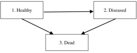
of analyzing incomplete data. Left censor, right censor, interval censor, and left truncation can happen, hence adding more difficulty to analyze the model and construct likelihood function (3). Censoring causes underestimate time to events. In some cases, it was assumed in this study that the censor and truncated data are independent of the process (4). In the present study, a 3-state illness-death (disability) model was considered with 3 transitions, which showed the progression of a disease (Figure 1). In this model, healthy individuals become diseased and then die or healthy individuals die because of other reasons.
Figure 1. Three state illness-death model
There are two important terms in this context, transition probability and transition intensity or transition rate.
A multi-state process is a stochastic process (X (t), t ∈ T) with a finite number of states S = {1, …, N}.
The time interval is T = [0, τ], τ < ∞ and state occupied at t is the value of time t. A multi-state process X (.) generates a history Ht-(ϭalgebra)
consisting of the observation of the process in the interval [t, ∞). In relative to this history, transition probabilities may be defined by the following relation:
Transition intensity displays potential hazard of progression to state j conditionally on occupying state h.
In this study, the focus is on the Markov and semi-Markov MSMs:
1) Markov models: Markov chain models
can accommodate censored data, competing risks (informative censoring), multiple outcomes, recurrent outcomes, frailty, and
inconstant survival probabilities (2). Future evolution depends on current state rather than the events occurred before the current state. In most applications, a Markov model is assumed for the MSMs (5). When there are covariates, a Cox (6) model is used to model the effect of covariates on each transition intensity.
2) Semi-Markov models: The future
evolution of the process does not depend on the current time but rather on the duration in the current state (7).
The goal in the present study was to fit MSMs and time dependent Cox regression model (CRM) on a time-to-event data and compare them.
Methods
The well-known cardiac allograft vasculopathy (CAV) dataset studied by Sharples et al. (8) were used in the present study. This dataset included 576 participants who received transplants between august 1979 to January 2000 and survived at least 1 year after transplantation and had undergone at least one coronary angiogram. The state at each time was a grade of CAV, a deterioration of the arterial walls (9). Approximately, each year after transplantation, each patient had an angiogram, at which CAV could be diagnosed. The result of the test was in the variable state, with possible values 1 and 2, representing CAV-free and CAV, respectively. A value of 3 was recorded at the date of death. Years designated the time of the test in years since the heart transplantation. Other variables included age (age at screen), donor age, and sex (0 and 1 representing men and women, respectively). Age and donor age were considered categorical, however the sex variable was dichotomous. Two cut points for age and donor’s age were taken into account mostly based on the quantiles. 30 and 50 were the cut points of age variable and for 20 and 40.
Time dependent CRM: In the analysis of
time-to-event data, the Cox proportional-hazards regression model has achieved popularity due to considering the censoring and the covariates. The Cox model with time-dependent covariate was much more complex than with fixed (time 1. Healthy
3. Dead
invariant) covariates due to the possibility of changing the values over time. This model involved constructing a function of time (10). The marginal distribution of survival times, that is, without consideration of CAV, was analyzed using the Cox proportional hazards regression model (6). Thus, the hazard function for individual i with covariates Zi was assumed to
have the following form with unspecified baseline hazard function α0(t) and regression
coefficients β.
The survival probability ̂ for given covariates of simple Cox model, Z, maybe estimated by
̂ ∏ ̂ ( ̂ )
Where, ̂ is the Breslow estimator for the integrated baseline hazard function.
Cox-Markov model (CMM): Finding a
relation between predictor variables and the response variable was one of the biggest goals of MSMs in the present study. This model have been used in literature to relate the individual characteristics to the intensity transition through a possibly time-dependent covariate vector Z (11). The simplest way was to decouple the whole process into several survival models. The illness-death model has been presented in figure 2, fitting separate intensity rates to all possible transitions using semi-parametric Cox proportional hazard regression models, while making appropriate adjustments to the risk set (7). Using Cox-like models of the form
, the transition
intensities for illness death model are
, (4). This model was
CMM which assumes the process to be Markovian. Estimating transition probability, taking into account independent z variables, yields:
̂ ∏ ∑ ̂
̂ ∏ ̂
̂ ∏ ̂ ̂
̂
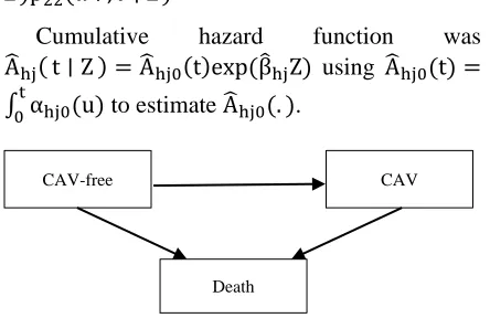
Cumulative hazard function was ̂ ̂ ̂ using ̂ ∫ to estimate ̂ .
Figure 2. A three-state model for the cardiac allograft vasculopathy (CAV) data
Cox semi-Markov model (CSMM): Markov
models have some limitations which hindered its use. Markov assumption was violated in some situations, meaning that the future depended on the individual's past only through his/her current state. In this model, the time was reset to zero when a new state was reached, hence the time scale was called “clock reset”. Each time the patient entered a new state, time was reset to 0. Therefore, CSMM could be easily fitted for the illness-death model; transition 2 → 3 was the difference between CMM and CSMM. The Markov assumption was not satisfied, as the mortality after getting CAV depended strongly on the time since getting CAV, suggesting that a semi-Markov model might be more appropriate (12). It was only needed to remodel α23, so that it
depended only on the duration in state 2. Using time since getting CAV as the basic time scale for the model for mortality after getting CAV, We model α23 as follows
( )
Where, t2i was the entry time into state 2. R
package p3state.msm was used for analyses. The significance level was considered to be 0.050 in this study.
Results
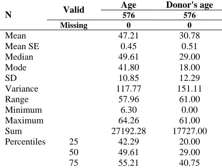
15% and 85% of the participants were women and men, respectively. The mean age of the
CAV-free
Death
individuals was 47 (47 and 43 for men and women, respectively). The mean age of donors was 30. The number of individuals suffering from CAV was 179 out of 576 (31.00%). Among the patients, 12 (14.46%) women and 167 (33.87%) men had CAV. Further information was listed in tables 1 and 2. During the study period, 576 individuals were at risk of transition from the state 1 to states 2 and 3 and transition from the state 2 to state 3. Of these, 179 (167 and 12 men and women, respectively) experienced a transition to the state 2, and 139 (120 and 19 men and women, respectively) to state 3.
Table 1. Continuous characteristics of the study variables
N Valid
Age Donor's age
576 576 Missing 0 0
Mean 47.21 30.78
Mean SE 0.45 0.51
Median 49.61 29.00
Mode 41.80 18.00
SD 10.85 12.29
Variance 117.77 151.11
Range 57.96 61.00
Minimum 6.30 0.00
Maximum 64.26 61.00
Sum 27192.28 17727.00
Percentiles 25 42.29 20.00
50 49.61 29.00
75 55.21 40.75
SE: Standard error; SD: Standard deviation
95 individuals (88 and 7 men and women, respectively) died without exposing to CAV. The number of individuals remaining in state 1 was 258. In addition, 84 of individuals were censored on transition from state 2.
The transition probabilities are changing over time. In the present study, transition probabilities were calculated only for median of
time in table 3, the probability of remaining CAV-free cases was 0.78. The estimated probability for individuals with transition from state 1 to state 2 was 0.14. For patients with CAV, there was a probability of 0.18 to die and the probability of dying because of reasons other than CAV was 0.08. Patients with CAV had a 0.82 probability to remain in state 2. It is noteworthy that these estimated transition probabilities were only valuable at median of time and they will change for other values of time (13).
Model fit
Time dependent CRM: In case of ignorance of the intermediate event, the results with time dependent CRM shown in table 4 indicated that only the individuals > 50 years old are significant (P = 0.0027). The individuals > 50 years old have 2.46 chance of death compared with those with < 30 years old.
Multi-State Models (MSMs)
Cox Markov Model (CMM): In transition from the state 1 to the state 2 as see in table 5, donor’s age variable for 20-40 years old donors was in borderline significance (P = 0.053), and for more than 40 years old, donors were highly significant (P < 0.001). Individuals with donors > 40 years old had a 2.233 chance of CAV compared to individuals with donors < 20 year old. The sex variable was significant as well (P = 0.030). Comparing to men, women had 0.518 hazard of CAV.
In transition from the state 1 to the state 3 in table 6, it was shown that the age variable for category of > 50 years old CAV-free individuals was significant (P < 0.001). Individuals > 50 years old had 3.652 chance of dying without getting CAV compared to < 30 year-old individuals.
Table 2. Table of frequencies
Without CAV CAV
Alive rate (%) Dead rate (%) Alive rate (%) Dead rate (%)
Sex Men 206 (63.2) 120 (36.8) 79 (47.3) 88 (52.7)
Women 52 (73.2) 19 (26.8) 5 (41.7) 7 (58.3)
Age (year)
< 30 27 (73.0) 10 (27.0) 8 (36.4) 14 (63.6) 30-50 99 (67.8) 47 (32.2) 41 (41.8) 57 (58.2) > 50 132 (61.7) 82 (38.3) 35 (59.3) 24 (40.7) Donor's age
(year)
Table 3. Transition probabilities for median of time State 1 State 2 State 3
State 1 0.78 0.14 0.08
State 2 0 0.82 0.18
The donor’s age > 40 years old was an important risk factor (P = 0.043). In addition, individuals with donor of > 40 years old had 1.665 chance of dying without getting CAV comparing to individuals with donor age of < 20 years old. Moreover, in transition from the state 2 to the state 3, there was no important risk factor depending on CMM.
Table 4. Time-dependent Cox regression model (CRM)
Coef Exp (coef)
Se
(coef) z P-value Lower Upper Factor
(age) 1
0.131 1.140 0.238 0.549 0.583 0.714 1.818
Factor (age) 2
0.901 2.463 0.247 3.646 0.000 1.517 3.998
Factor (dage) 1
0.076 1.079 0.170 0.445 0.657 0.773 1.505
Factor (dage) 2
0.201 1.222 0.201 1.000 0.317 0.825 1.811
Sex 0.399 1.490 0.218 1.831 0.067 0.972 2.283 Treat 1.013 2.754 0.160 6.340 < 0.001 2.014 3.767
Likelihood ratio test = 69.01099 on 6 df, P < 0.001 -2 * Log-likelihood = 2358.093
dage: Donor’s age
Cox Semi Markov Model (CSMM): Markov assumption should only check for transition from 2 to 3 in the illness-death model. The Markov assumption was highly significant in the present study (P = 2.27e-11).
Table 5. Cox Markov Model (CMM) transition from state 1 to state 2
Coef Exp (coef)
Se
(coef) z P-value l u Factor
(age) 1
0.189 1.208 0.242 0.780 0.435 0.751 1.943
Factor (age) 2
-0.142 0.867 0.261 -0.546 0.585 0.520 1.446
Factor (dage) 1
0.390 1.476 0.202 1.928 0.054 0.993 2.194
Factor (dage) 2
0.803 2.233 0.229 3.515 < 0.001 1.427 3.495
Sex -0.657 0.519 0.304 -2.161 0.031 0.286 0.941 dage: Donor’s age
Likelihood ratio test = 22.85106 on 5 df, P < 0.001 -2 * Log-likelihood = 1904.55
Table 6. Cox Markov Model (CMM) transition from state 2 to state 3
Coef Exp (coef)
Se
(coef) z P-value l u Factor
(age) 1
0.436 1.547 0.359 1.216 0.224 0.766 3.127
Factor (age) 2
1.295 3.652 0.357 3.632 < 0.001 1.815 7.347
Factor (dage) 1
0.164 1.178 0.224 0.732 0.464 0.759 1.829
Factor (dage) 2
0.510 1.665 0.252 2.025 0.043 1.017 2.726
Sex 0.368 1.445 0.256 1.436 0.151 0.874 2.389 dage: Donor’s age
Likelihood ratio test = 37.28319 on 5 df, P < 0.001 -2 * Log-likelihood= 1444.886
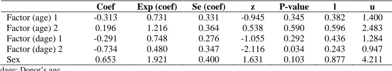
This assumption was tested in table 7, showing that the transition rates in states were affected by the previous sojourn time. Therefore, CSMMs could be a better choice. This model was fitted only for transition from the state 2 to the state 3. Results in table 8 indicated that the donor’s age > 40 years old was significant (P = 0.034). Patients with CAV with donor’s age of > 40 year old had 0.48 chance of death compared to the patients with CAV with donor’s of < 20 years old.
Table 7. Markov assumption test
Coef Exp (coef)
Se
(coef) z P-value Factor
(age) 1
-0.398 0.672 0.330 -1.210 0.227
Factor (age) 2
0.280 1.323 0.359 0.780 0.435
Factor (dage) 1
-0.238 0.788 0.284 -0.840 0.400
Factor (dage) 2
-0.753 0.471 0.356 -2.110 0.035
Sex 0.787 2.197 0.409 1.920 0.054 Start -0.292 0.747 0.046 -6.280 < 0.001 dage: Donor’s age
Likelihood ratio test = 61.5 on 6 df, P < 0.001 n = 179, number of events = 95
Discussion
Table 8. Cox Semi-Markov Model (CSMM) from state 2 to state 3
Coef Exp (coef) Se (coef) z P-value l u Factor (age) 1 -0.313 0.731 0.331 -0.945 0.345 0.382 1.400 Factor (age) 2 0.196 1.216 0.364 0.538 0.590 0.596 2.483 Factor (dage) 1 -0.291 0.748 0.276 -1.055 0.292 0.436 1.284 Factor (dage) 2 -0.734 0.480 0.347 -2.116 0.034 0.243 0.947
Sex 0.653 1.921 0.400 1.631 0.103 0.877 4.211
dage: Donor’s age
Likelihood ratio test = 9.381181 on 5 df, P = 0.095 -2 * Log-likelihood = 708.6002
In this study, the use of MSMs in the analysis of survival data were discussed in the scope of the three-state model. Nonparametric estimators for the transition probabilities have been presented and illustrated using a real dataset on CAV. The first model, a Markov process model did not fit the data since the mortality after CAV depended strongly on the time since CAV, and, instead, semi-Markov model was studied. These three-state models turned out to provide important clinical information by highlighting covariates affecting the mortality and covariates affecting the CAV. The main message of this study, however, is the fact that the precision of survival probability estimates based on the three-state models tended to be better than for those based on the simple Cox model. As it can be seen in the results, there are different risk factors affecting every single transitions. However, the result of simple CRM is not precise as MSMs.
Conclusion
In conclusion, the present study has shown that a MSM may in some cases be preferable to a model for the marginal survival distribution. Thus, for the MSM to be analyzed simply, exact times of transition are required when the observation of some transition times are interval-censored, hence the likelihood expressions become more involved.
Moreover, the multi-state analysis requires some assumptions concerning a Markov or semi-Markov structure of the data assumptions which are avoided in the marginal analysis (14). Final problem with the MSMs is that estimates for transition probabilities are not generally available for semi-Markov models. At last, it is important to realize that there are several
modelling strategies for the intermediate event and that each of these strategies has restrictions and may cause different results.
Conflict of Interests
Authors have no conflict of interests.
Acknowledgments
We would like to thank all of the colleagues of Department of Epidemiology and Biostatistics, Tehran University of Medical Sciences, Iran, who supported this study.
References
1. Andersen PK, Esbjerg S, Sorensen TI. Multi-state models for bleeding episodes and mortality in liver cirrhosis. Stat Med 2000; 19(4): 587-99.
2. Abner EL, Charnigo RJ, Kryscio RJ. Markov chains and semi-Markov models in time-to-event analysis. J Biom Biostat 2013; Suppl 1(e001): 19522.
3. Commenges D. Inference for multi-state models from interval-censored data. Stat Methods Med Res 2002; 11(2): 167-82. 4. Meira-Machado L, de Una-Alvarez J,
Cadarso-Suarez C, Andersen PK. Multi-state models for the analysis of time-to-event data. Stat Methods Med Res 2009; 18(2): 195-222. 5. Kay R. A Markov model for analyzing cancer
markers and disease states in survival studies. Biometrics 1986; 42(4): 855-65.
6. Cox DR. Regression models and life-tables. J R Stat Soc Series B 1972; 34(2): 187-220. 7. Meira-Machado L, Roca-Pardinas R.
Wallwork J, Large SR. Diagnostic accuracy of coronary angiography and risk factors for post-heart-transplant cardiac allograft vasculopathy. Transplantation 2003; 76(4): 679-82.
9. Jackson C. Multi-state modelling with R: The msm package. J Stat Softw 2011; 38(8): 1-29. 10. Fisher LD, Lin DY. Time-dependent covariates in the Cox proportional-hazards regression model. Annu Rev Public Health 1999; 20: 145-57.
11. Heutte N, Huber-Carol C. Semi-markov models for quality of life data with censoring. In: Mesbah M, Cole BF, Lee MT, Editors.
Statistical methods for quality of life studies. Berlin, Germany: Springer Science & Business Media, 2002. p. 207-18.
12. Shu Y, Klein JP, Zhang MJ. Asymptotic theory for the Cox semi-Markov illness-death model. Lifetime Data Anal 2007; 13(1): 91-117.
13. Titman AC. Transition probability estimates for non-Markov multi-state models. Biometrics 2015; 71(4): 1034-41.