Gabriel Caloz & Monique Dauge, Editors
FINITE ELEMENT METHOD WITH PATCHES FOR POISSON PROBLEMS IN
POLYGONAL DOMAINS
Alexei Lozinski
1, Jacques Rappaz
2and Jo¨
el Wagner
3Dedicated to Prof. Michel Crouzeix
Abstract. In this paper we consider the finite element approximation of the singularities of the solution of Poisson problems in a polygonal domain with reentrant corners or changing Dirichlet-Neumann boundary conditions. We use a correction algorithm with patches of elements to improve the a priori error estimates and to obtain the same order as the optimal estimate when everything is regular. We give an application of the correction method to the problem of glacier modeling.
Introduction
The aim of this paper is to use the finite element method with patches, introduced by Glowinski et al. in [11, 12], in the setting of certain problems with singular solutions as studied for example by Raugel [20] and Grisvard [15, 16], earlier by Babuska [1], and after by Dauge [8], Brenner [4], Cai et al. [5]. The results of this paper have first been presented by Wagner in [22] but we give here some simpler and more general proofs for them.
A method for the numerical solution of elliptic problems with multi-scale data using multiple levels of not necessarily nested grids is introduced in [12] and analyzed in [11]. We recall this algorithm here for the conve-nience of the reader. The method consists in calculating successive corrections to the solution in patches whose shape is not necessarily conforming with the global coarse grid. We consider a polygonal domain Ω⊂R2 with boundary ∂Ω split into two parts Γ1, Γ2, and V ={v ∈H1(Ω) such thatv = 0 on Γ1} where H1(Ω) denotes the usual Sobolev space of functions with first derivatives inL2(Ω). Leta:V×V →Rbe a bilinear, symmetric, continuous and coercive form. Iff ∈L2(Ω), we are looking for the uniqueu∈V such that
a(u, v) =
Z
Ω
f vdx, ∀v∈V. (1)
An approximation of u by the finite element method of order r consists in introducing a regular family of triangulationsTH of Ω [6, Sect. 17], defining
VH = {g: Ω→Rcontinuous such that g|K∈Pr(K),∀K∈ TH andg= 0 on Γ1},
1
Dept. of Mathematics, University of Houston, 4800 Calhoun Road, Houston, Texas 77204-3008, USA ([email protected]).
2
Section of Mathematics, Ecole Polytechnique F´ed´erale de Lausanne (EPFL), 1015 Lausanne, Switzerland ([email protected]).
3
c
EDP Sciences, SMAI 2007
wherePr(K) is the space of polynomials of degree≤ron triangleK∈ TH, and calculating uH ∈VH satisfying
a(uH, v) =RΩf vdx,∀v ∈VH. Consider now Λ⊂Ω another open polygonal domain wherein we would like to obtain a better precision on the solutionuthan the one given by uH. Take note that Λ is not necessarily the union of several trianglesK ofTH. LetTh be a regular family of triangulations of Λ and consider
Vh = {g: Ω→Rcontinuous such that g|K ∈Ps(K),∀K∈ Th andg= 0 on Ω\Λ, g= 0 on Γ1}.
We callH = maxK∈THdiam(K) and h= maxK∈Thdiam(K). Setting VHh =VH+Vh as approximation foru we are looking for the function uHh ∈VHh satisfying
a(uHh, v) =
Z
Ω
f vdx, ∀v∈VHh. (2)
Remark that, in general, VHh is not a direct sum ofVH and Vh. In practice, it is not possible to determine a finite element basis of VHh and hence to compute directly uHh. It is the reason why we use the following algorithm for computinguHh: At iterationn= 0 we initialize withu0
H =uH, u0h = 0 and choose a relaxation parameterω ∈(0; 2). Then forn= 1,2,3, . . . we writeun−1=un−1
H +u n−1 h withu
n−1
H ∈VH,unh−1∈Vh. We write the first step of then-th iteration of the algorithm as follows:
Find vh∈Vhs.t. a(vh, ϕ) =RΩf ϕdx−a(unH−1, ϕ), ∀ϕ∈Vh . Setun
h= (1−ω)u n−1 h +ωvh.
The same holds for the second step which writes out explicitly: Find vH∈VH s.t. a(vH, ϕ) =RΩf ϕdx−a(unh, ϕ), ∀ϕ∈VH. Setun
H= (1−ω)u n−1
H +ωvH. Remark thatun
h=u n−1
h +ωwh wherewh∈Vhis such that
a(wh, ϕ) =RΩf ϕdx−a(unH−1+u n−1
h , ϕ), ∀ϕ∈Vh, and that un
H =unH−1+ωwH where wH ∈VH is such that
a(wH, ϕ) =RΩf ϕdx−a(uHn−1+unh, ϕ), ∀ϕ∈VH. In [11] it is proven that un converges to u
Hh when n tends to infinity and, provided u ∈ Hq(Ω) with q = max(r, s) + 1, the approximationuHh tousatisfies thea priori error estimate
||u−uHh|| ≤CHr||u||Hq(Ω\Λ)+hs||u||Hq(Λ)
, (3)
whereC is a constant independent ofH andh, and||v||=a(v, v)1/2,∀v∈V.
At this point, taking inspiration from the described correction method we consider regularity and convergence results for problems with singularities due to changing Dirichlet-Neumann boundary conditions and domains with reentrant corners. Such problems have been studied for example by Raugel [20] and Grisvard [15, 16].
1.
Preliminary results
In this section we introduce an estimate (Proposition 1.3) for the finite element interpolation on two super-imposed but not necessarily nested grids in a two-dimensional polygonal domain Ω of the function
ϕ=rγg(θ) (4)
where r, θ are the polar coordinates, 0< γ <1 is a number andg(θ)∈C∞([0,2π]) is a given function. We
suppose from now on that Ω does not contain the rayθ = 0 but Ω contains the origin, hence the function ϕ
does not belong to H2(Ω) and we cannot expect to find a finite element approximation of ϕwhich is order 1 accurate inH1 norm on a general grid.
Let Ca denote the intersection of Ω with the open disc of radius a > 0 centered at 0. We have for any
a∈(0, R) whereRis the radius of the smallest disc centered at the origin that contains Ω:
|ϕ|2H2(Ω\C
a)≤C Z 2π
0
Z R
a
r2γ−4(g(θ)2+g′(θ)2+g′′(θ)2)rdrdθ≤ a2C−2γ||g|| 2 H2([0,2π])
hence
|ϕ|H2(Ω\Ca)≤ C
a1−γ||g||H2([0,2π]) (5)
with constantCdepending only on γ. By a similar calculation, we have
|ϕ|H1(Ca)≤Caγ||g||H1([0,2π]) (6)
Lemma 1.1. For the setting above, function ϕ given by (4) and any a ∈(0, R), there exists a function ϕ˜ ∈
H2(Ω)such that ϕ˜|
Ω\Ca=ϕ|Ω\Ca and
|ϕ˜|H2(Ω)≤ C
a1−γ||g||H2([0,2π]) (7)
|ϕ˜|H1(C
a)≤Ca γ
||g||H1([0,2π]) (8)
with a constantC depending only on γ. If g(θ0) = 0 for some θ0 then ϕ˜ can be chosen so that it vanishes on
the ray θ=θ0.
Proof. Let us pick a functionχ∈C2([0,1]) such that
χ(0) = 0, χ′(0) = 0, χ(1) = 1, χ′(1) =γ
and define ˜ϕby
˜
ϕ=
ϕin Ω\Ca,
aγχ(r
a)g(θ) in Ca
We have then ˜ϕ∈H2(Ω) and |ϕ˜|H2(Ω\Ca)≤Caγ−1||g||H2([0,2π]) by (5). By change of variablesr→r/a, it is easy to see that the analogous estimate holds insideCa, namely|ϕ˜|H2(Ca)≤Caγ−1||g||H2([0,2π]), hence (7). The
estimate (8) follows in the same manner.
We introduce TH a regular family of triangulations (see Ciarlet [6, Sect. 17]) with triangles K over Ω and callH = maxK∈THdiam(K). We suppose that0is a node ofTH. LetrH be the standard nodal interpolant by piecewise linear functions onTH. Let moreover Γ be a (possibly empty) part of∂Ω consisting of several straight segments of non zero length starting from the origin and suppose that ϕof (4) vanishes on Γ. Consider the standard finite element space
VH = {g∈C0(Ω) such that g|K ∈P1(K),∀K∈ TH
We recall the following result [3, Theorem 6.3], which we prove here for completeness of exposition.
Lemma 1.2. There exists an element ϕH∈VH such that
|ϕ−ϕH|H1(Ω)≤CHγ||g||H2([0,2π]) (10)
whereϕis defined by (4) and C is a constant depending only onγ and the regularity parameter ofTH.
Proof. Take ϕH =rHϕ˜ where ˜ϕis the function constructed in Lemma 1.1 fora=H. Note that ˜ϕ|Γ = 0 and thereforeϕH ∈VH. Indeed, each segment from Γ lies on the rayθ=θ0 for someθ0. The functionϕcan vanish on such a segment only ifg(θ0) = 0, meaning that ˜ϕvanishes on this segment as well. We estimate now
|ϕ˜−ϕH|H1(Ω)≤CH|ϕ˜|H2(Ω)≤CHγ||g||H2([0,2π])
by standard approximation results from [6] and (7). Furthermore,
|ϕ−ϕH|H1(Ω)≤ |ϕ˜−ϕH|H1(Ω)+|ϕ|H1(CH)+|ϕ˜|H1(CH)≤CHγ||g||H2([0,2π])
by (6) and (8). Hence (10) is recovered.
Let us now consider a family of domains Λǫ⊂Ω such thatCǫ⊂Λǫ and introduce regular triangulationsTh on Λǫwithh= maxK∈Thdiam(K)≤ǫ. As before, we suppose that0is a node ofThand letrh be the standard nodal interpolant by piecewise linear functions onTh. Introduce the standard finite element space onTh:
Vh = {g∈C0(Ω) such that g|K ∈P1(K),∀K∈ Th
andg= 0 on Ω\Λǫ and on Γ}, (11)
Proposition 1.3. There exists an element ϕHh∈VH+Vh such that |ϕ−ϕHh|H1(Ω)≤C
H
ǫ1−γ +h γ
||g||H2([0,2π]) (12)
whereϕis defined by (4) and C is a constant independent ofH,h,ǫandg.
Proof. Let ˜ϕbe the function constructed in Lemma 1.1 for a=ǫ. We takeϕH =rHϕ˜ and assure ourselves that ϕH ∈ VH as in the proof of Lemma 1.2. Let us now apply Lemma 1.2 on Th instead of TH to construct
ϕh∈Wh={g∈C0(Λǫ) :g|K∈P1(K),∀K∈ Thand g= 0 on Γ}, for which we have
|ϕ−ϕh|H1(Λ
ǫ)≤Ch γ
||g||H2([0,2π]). (13)
It is easy to see that rhϕ˜∈Wh and, by construction, ϕh|∂Λǫ∩Ω =rhϕ|∂Λǫ∩Ω=rhϕ˜|∂Λǫ∩Ω. Consequently, we can takeψh∈Vh such thatψh|Λǫ=ϕh−rhϕ˜and setϕHh =ϕH+ψh. We estimate then
|ϕ−ϕHh|H1(Ω)≤ |ϕ˜−ϕH|H1(Ω)+|ϕ−ϕ˜−ψh|H1(Λǫ).
But
|ϕ˜−ϕH|H1(Ω)≤CH|ϕ˜|H2(Ω)≤C H
ǫ1−γ||g||H2([0,2π]) by standard approximation results from [6] and (7). Furthermore,
|ϕ−ϕ˜−ψh|H1(Λ
ǫ)≤ |ϕ−ϕh|H1(Λǫ)+|ϕ˜−rhϕ˜|H1(Λǫ) ≤Chγ||g||H
2([0,2π])+Ch|ϕ˜|H2(Ω)≤C
hγ+ h
ǫ1−γ
||g||H2([0,2π])
2.
Problem with change in boundary conditions
The objective of this discussion is to use the correction algorithm described in the Introduction on a Poisson problem with changing Dirichlet-Neumann boundary conditions. We first recall the regularity of the solution to such a problem and give thea priori convergence results. Next we implement the problem numerically, and after comparing the theoretical orders with the ones we obtain numerically, we use different types of patches in order to improve the convergence order.
2.1.
Regularity result.
Before introducing a model problem, see (19), we recall the analysis of the singular behavior as presented by Grisvard in [15, Section 4.4] and [16, Pages 49–51 and Section 2.4] through the following situation.
Consider the domain Ω∞ = (−∞; +∞)×(0; +∞). In all the following we set Hlocm(Ω∞) = {f : Ω∞ →
Rsuch thatf ∈ Hm(ω◦) for any compact setω ⊂ Ω∞,ω◦ 6= ∅its interior}. With this notation we consider the problem of finding the functions v ∈ H1
loc(Ω∞) verifying ∆v = 0 in Ω∞ and obeying the following set of
boundary conditions:
∂v
∂n = 0 on (−∞; 0)× {0}, and
v= 0 on (0; +∞)× {0}. (14)
We denote x1 andx2 the two space variables and (r, θ) are the polar coordinates. The situation as well as the notation used are illustrated in Figure 1.
O
x1 x2
r
∂v
∂n = 0 v= 0
er eθ
θ
Ω∞
Figure 1. Illustration of the situation and notation.
To analyze these solutions, we consider the function v =v(r, θ) in polar coordinates. Taking into account the boundary conditions, we write
v(r, θ) = X m≥0
ρm(r) sin
2m+ 1
2 θ
, (15)
and calculate its gradient and Laplacian. If we assume ρm(r) = cmrγ, the harmonic functions in Ω∞ with
boundary conditions (14) are expressed in polar coordinates by
v(r, θ) = X m≥0
cmr(2m+1)/2+c−mr−(2m+1)/2
sin
2m+ 1
2 θ
, (16)
wherecm,c−mare real coefficients. Note thatc0andc−0are different a priori. Using the general expression (16) in polar coordinates, we analyze the regularity of these solutions. For |∇v|2 to be locally integrable in Ω
∞ a
0
−L L
0
l
Γ2 Γ1
Γ3 Ω
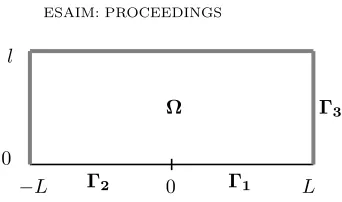
Figure 2. Illustration of the domain Ω and its boundaries Γi,i= 1,2,3.
the functions of the form (16) that areH1
loc(Ω∞) are expressed by
v(r, θ) = X m≥0
cmr(2m+1)/2sin
2m+ 1
2 θ
. (17)
Furthermore, considering the second derivatives of v, we note that, if c0 6= 0, then v does not belong to Hloc2 (Ω∞).
Thus we are interested in calculatingpsuch thatv of the form (17) withc06= 0 is inWloc2,p(Ω∞). For finding
suchp, we evaluate the second derivative ofr1/2sin(θ/2) (c
06= 0) and require it to bep-integrable with measure rdrdθ. We obtain the relation−3
2p+ 1>−1, and hencep < 4 3. In conclusion, if v∈H1
loc(Ω∞) is an harmonic function in Ω∞ verifying the boundary conditions (14), then v∈Wloc2,p(Ω∞) withp∈[1;43). We denote by ϕ(r, θ) the componentm= 0 ofv,
ϕ(r, θ) =c0√rsin(θ/2). (18)
2.2.
Model problem and
a priori
error estimate.
Let now Ω = (−L;L)×(0;l)⊂R2be a rectangular domain (see Figure 2). We consider the following Poisson problem with homogeneous Dirichlet-Neumann boundary conditions:
For givenf ∈L2(Ω), findu∈H1(Ω) such that
−∆u=f in Ω,
u= 0 on Γ1={(x1,0) : 0< x1< L}, ∂u
∂n = 0 on Γ2={(x1,0) :−L < x1<0},
u= 0 on Γ3=∂Ω\(Γ1∪Γ2).
(19)
Let us remark that this problem means that, ifV ={v∈H1(Ω) :v= 0 on Γ
1∪Γ3}, thenu∈V satisfies
Z
Ω∇
u· ∇vdx=
Z
Ω
f vdx, ∀v∈V. (20)
Thanks to Grisvard [16, Section 2.4] complemented by the above paragraph, and since the four corners of Ω are right angles, we know that the unique solution u of (20) (Lax-Milgram Theorem) can be written as
u=w+ϕwherew∈H2(Ω) andϕis given by (18).
Recall thatTH denotes a regular triangulation over Ω with trianglesK. We require that the origin be a node ofTH. LetuH ∈VH={ψ∈C0(Ω) : ψ|K ∈P1(K),∀K∈ TH andψ= 0 on Γ1∪Γ3}be the approximation ofu
such that Z
Ω∇
uH· ∇vHdx=
Z
Ω
f vHdx, ∀vH ∈VH. (21)
Using C´ea’s Lemma we haveR
Ω|∇(u−uH)|
2dx=R
takingvH =rHw+ϕHwhereϕH ∈VHis the function constructed in Lemma 1.2,|u−uH|H1(Ω)≤ |u−rHu|H1(Ω). By Lemma 1.2 and standard interpolation results we have the followinga priori error estimate:
||u−uH||H1(Ω)≤C(c0H 1
2 +H|w|H2(Ω)), (22)
whereC is a constant independent ofH andu. Hence, thea priori convergence order in H in the H1-norm is only of order 1/2.
The objective of the next part will be to apply the correction method to the present situation. We use a patch Λ with a finer triangulation to augment the precision around the origin where the first derivative of the solutionuexplodes inO. By strategically choosing the patch we try to optimize the convergence order.
2.3.
Improving the
a priori
convergence order through using patches.
In this paragraph we keep considering the model problem (19) introduced above with its approximation (21). The aim is to use the correction algorithm to obtain a bettera priori convergence order.
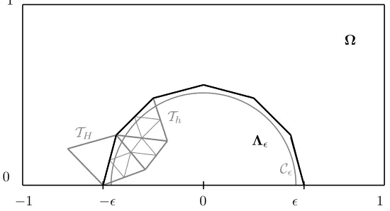
We consider two families of regular triangulations TH over Ω and Th over a patch Λǫ, the size of which depends on ǫ > 0 in the sense that Λǫ ⊃Cǫ. We suppose that Λǫ∩Γ3 = ∅, see Figure 3 with L = l = 1. Then the idea is to use piecewise polynomial functions of degree 1 onK∈ TH resp. Th, and to approximate the solutionuof (19) withuHh=uH+uh,uH anduhdefined onTH andThby the correction algorithm described in the Introduction. More precisely, we keep the finite element spaceVH from the preceding section, and we introduce the new one
Vh={ψ∈H1(Ω) : ψ|K ∈P1(K),∀K∈ Th andψ= 0 in Ω\Λǫ andψ= 0 on Γ1∩∂Λǫ)}
TH
Th
0
−1 1
0 1
−ǫ ǫ
Ω
Cǫ Λǫ
Figure 3. Illustration of the setting and notation.
Proposition 2.1. If u is the solution of (19) and if 0 is a node of both TH and Th then there exists C
(independent ofH,handǫ) such that the approximationuHh defined by (2) satisfies the a priorierror estimate
|u−uHh|H1(Ω)≤C
H
√ǫ+√h
. (23)
Proof. Sinceuis the solution of (19) we have thatu=w+ϕ, wherew∈V∩H2(Ω) andϕis given by (18), i.e. ϕ=c0√rsin(θ/2). Hence we obtain by using C´ea’s Lemma, i.e. |u−uHh|H1(Ω)≤ |u−vHh|H1(Ω),∀vHh ∈VHh,
where ϕHh is the function constructed in Proposition 1.3 withγ= 12 in (4) and Γ = Γ1 in (9) and (11). Note that rHw|Γ1 =ϕHh|Γ1 = 0 andrHw|Γ3 =−rHϕ|Γ3=−ϕHh|Γ3, so indeedrHw+ϕHh∈VHh.
Standard interpolation results yield
|w−rHw|H1(Ω)≤CH|w|H2(Ω) (25)
and we conclude by applying the estimate (12).
It is of interest to write out in Proposition 2.1 the caseǫ=αHβ, whereαandβ denote constants,β <1:
|u−uHh|H1(Ω)∼
H1−β/2+h1/2. (26)
In the case whereβ = 0, i.e. the patch is fixed (ǫ=α), we note that convergence of order one inH can be obtained when choosinghproportional to H2. It is adequate to note here that Grisvard proves, under certain conditions [15, Theorem 8.4.1.6] on the local refinement of a family of triangulations, that optimal convergence order, i.e. order one inH1(Ω)-norm, can be reached despite the singularity [15, Corollary 8.4.1.7]. In the present situation of a solution inW2,p(Ω) with p∈[1;4
3), the conditions of Grisvard’s Theorem 8.4.1.6 [15] aim that, as H→0, there exists a constantσsuch that
(i) maxK∈THHK/ρK≤σwhereHK is the diameter andρK the interior diameter ofK, i.e., the family of triangulations is regular;
(ii) HK≤σH2, for any triangleK with one corner at the origin; (iii) HK≤σHinfKr1/2, for any triangleK without corner at the origin.
Condition (ii) of the above result on the refined families requires that the diameter of triangles around the origin is of orderH2. The above discussion of Proposition 2.1 also implies this crucial condition which can also be found in the work [20] by Raugel.
We remark that if ǫ=H, (26) becomes |u−uHh|H1(Ω)∼( √
H+√h), which leads to an estimate O(√H) whenh=H, showing that such a patch is useless.
As we will see in the sequel, it is of practical interest to choose patches of variable size when refining, in particular with respect to memory usage and computation time.
2.4.
Numerical results.
In order to assess the given error estimate, we consider the problem of approximatingu=w+ϕwithw= 0 and ϕ given by (18). We consider the geometry illustrated in Figure 2. Numerical tests when solving the problem of findingu∈H1(Ω) such that
−∆u= 0 in Ω,
u= 0 on Γ1,
∂u
∂n = 0 on Γ2,
u=ϕ|Γ3 on Γ3,
(27)
yielding obviouslyu=ϕ, are reported in the following. An illustration of the isolines of the solutionu=ϕis given in Figure 4.
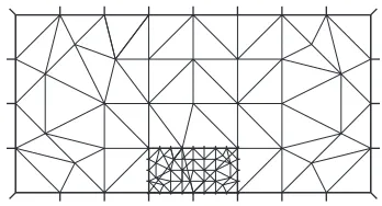
Over Ω = [−L;L]×[0;l] with L = l = 1 we consider an unstructured regular triangulation TH using a discretization of (−L;L) withN intervals and (0;l) with N/2 intervals. We choose Λǫ = (−ǫ;ǫ)×(0;ǫ) and considerTh a regular and unstructured triangulation based on a discretization of (−ǫ;ǫ) withM intervals and (0;ǫ) withM/2 intervals. In Figure 5 we illustrate the grid constellation withǫ= 0.25 andN =M = 8.
Accordingly with the discussion at the end of the last paragraph, we chooseǫ=αHβ,β <1, andh=H2−β so that the two terms in (26) are of the same order inH. With the above notation this is obtained when choosing
IsoValue 0
0.05
0.1
0.15
0.2
0.25
0.3
0.35 0.4 0.45 0.5 0.55 0.6 0.65 0.7 0.75 0.8 0.85 0.9 0.95 1
Figure 4. Isolines of the solutionu=ϕof problem (27).
Figure 5. Grid constellation showing a patch withǫ= 0.25 andN =M = 8.
α β ǫ h M CO1 CO2
0.25 0 0.25 H2 N2/32 1 1.06
1 1/4 H1/4 H7/4 N3/2/√2 7/8 = 0.875 0.85 1 1/2 √H H3/2 N 3/4 = 0.750 0.72 1 3/4 H3/4 H5/4 N1/2√2 5/8 = 0.625 0.61
no patch 0.5 0.50
Table 1. Synoptic table of chosen patches and H1(Ω)-norm convergence orders (CO1 =a priori order inH, CO2 = order obtained by numerical experience).
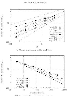
of different cases of patch size in function ofH applied on the solution of problem (27) is reported in Table 1. In the last column of the latter we report the numerically obtained order inH. This value corresponds to the slope (in logarithmic scale) at the last level of refinement of the decreasing relative H1(Ω)-norm error in the mesh sizeH. This is readily seen from Figure 6(a) where we illustrate the concluding convergence behavior in the mesh-size graphically.
slope 1/2 slope 3/4slope 1 no patch ǫǫ==H3/4 √
H ǫǫ== 0.25H1/4
H
R
el
a
ti
v
e
H
1-n
o
rm
er
ro
r
eH
h
0.1 0.01
0.1
0.01
(a) Convergence order in the mesh size.
no patch ǫ=ǫ=H0.75 √
H ǫǫ== 0.25H0.25
Number of nodes
R
el
a
ti
v
e
H
1-n
o
rm
er
ro
r
eH
h
100000 10000
1000 100
10 0.1
0.01
(b) Error reduction vs. number of nodes.
Figure 6. Convergence ofuH resp. uHh touwith respect to the mesh sizeH and the number of nodes.
The results of this model problem with a singularity due to the change in the boundary conditions are transferable to singularities whose origin lies in a computational domain with reentrant corner. This study is presented in the next section.
3.
Problem in a domain with reentrant corner
In the previous section we have discussed the Poisson problem in a rectangular domain with changing Dirichlet-Neumann boundary conditions. In the sequel, the objective is to examine a Poisson-Dirichlet problem in domains with reentrant corners. This will be done similarly to the foregoing analysis.
3.1.
Regularity result.
A brief analysis of this situation can be found in Grisvard [15, Sections 4.4 and 8.4] and [16, Pages 49–51 and Section 2.4]. It is useful to recall the results here.
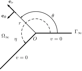
Consider the domain Ω∞⊂R2as depicted in Figure 7. We consider for Ω∞the part ofR2where the internal
functions v∈H1
loc(Ω∞) verifying ∆v= 0 in Ω∞ with homogeneous Dirichlet boundary conditions on Γ∞. We
consider polar coordinates centered at the corner O of Γ∞. The situation and the notation are illustrated in
Figure 7.
O r
Γ∞ v= 0
v= 0 er
eθ θ
Ω∞ η
Figure 7. Illustration of the situation and notation.
We follow the same analysis of the solution as in the previous section. Taking into account the shape of the domain and the boundary conditions, we consider the functionv =v(r, θ) of the form
v(r, θ) = X m≥1
ρm(r) sin
mπ ηθ
. (28)
With the same techniques we show that ρm(r) is of the formcmrmπ/η for obtainingv∈Hloc1 (Ω∞).
Considering the second derivatives ofv, we note that, ifc16= 0, thenv does not belong toHloc2 (Ω∞). Thus
we are interested in calculating psuch that v withc16= 0 is in Wloc2,p(Ω∞). For finding suchp, we evaluate the
second derivative ofrπ/η(c
16= 0) and require it to bep-integrable. We obtain the relation
π η −2
p+ 1>−1, and hencep < 2−2π/η.
In conclusion, ifv∈H1
loc(Ω∞) is an harmonic function in Ω∞verifying the homogeneous Dirichlet boundary
condition on Γ∞, thenv∈Wloc2,p(Ω∞) withp∈[1;2−2π/η). Note that in the extremal case whereη→2πwe are
left with Wloc2,p-regularity,p∈[1;43). Thus the regularity of this extreme situation in the current problem of a domain with reentrant corner corresponds to the regularity of the problem with changing Dirichlet-Neumann boundary conditions on a straight boundary as studied in Section 2.
3.2.
Model problem and
a priori
error estimate.
Let the domain Ω ⊂ (−L;L)2 ⊂ R2 be the L-shaped domain as depicted in Figure 8. We consider the following Poisson problem with homogeneous Dirichlet boundary conditions:
For givenf ∈L2(Ω), findu∈H1(Ω) such that
−∆u=f in Ω,
u= 0 on∂Ω. (29)
Thanks to Grisvard [16, Section 2.4] complemented by the above paragraph withη = 3π/2, we know that the unique solutionuof (29) can be written asu=w+ϕwhere w∈H2(Ω) and
(0,0)
(−L,−L) (L,−L)
(−L, L)
Ω Γ
Figure 8. Illustration of the domain Ω.
Recall that TH denotes a regular triangulation over Ω with triangles K. We call H = maxK∈THdiam(K). By Proposition 1.2 we have the followinga priori error estimate:
|u−uH|H1(Ω)≤C(c0H 2
3 +H|w|H2(Ω)), (31)
whereC is a constant independent ofH andu. Hence, thea priori convergence order in H in the H1-norm is only 2/3.
3.3.
Improving the
a priori
convergence order through using patches.
In this section we keep considering the model problem (29) introduced above. The aim is to use the correction algorithm to obtain a bettera priori convergence order. Complete analysis alike in Section 2 can be performed and leads to a particular result similar to Proposition 2.1 adapted to the current problem. We will not reiterate such a reasoning here.
Consider two families of regular triangulations TH over Ω (as above) and Th over Λǫ, Λǫ = (−ǫ;ǫ)2∩Ω. Recall thatH = maxK∈THdiam(K) and callh= maxK∈Thdiam(K) the diameter of the trianglesK. We use hat function elements and approximate the solutionuof (29) withuHh=uH+uh,uHanduhdefined by using TH andTh respectively and by using the correction method given in the Introduction.
We are able to prove in the same way as Proposition 2.1 that there exists C such that the approximation
uHh tousatisfies thea priori error estimate
|u−uHh|H1(Ω)≤C
H ǫ1/3+h
2/3
. (32)
It is of interest to write out (32) whenǫ=αHβ, whereαandβ denote constants,β <1:
|u−uHh|H1(Ω)∼
H1−β/3+h2/3. (33)
IsoValue
0 0.05
0.1
0.15 0.2 0.25 0.3 0.35 0.4 0.45 0.5 0.55 0.6 0.65 0.7
0.75
0.8 0.85 0.9 0.95 1
1.05
1.1
1.15
1.2
Figure 9. Isolines of the solutionu=ϕof problem (34).
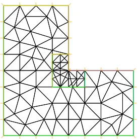
Figure 10. Illustration of the used grid constellation withǫ= 0.25 andN = 8,M = 4.
3.4.
Numerical results.
In order to assess the given error estimates, we consider the problem of approximatingu=w+ϕwithw= 0 andϕgiven by 30. Numerical tests when solving the problem of findingu∈H1(Ω) such that
−∆u= 0 in Ω, u=ϕ|∂Ω on∂Ω,
(34)
yielding obviouslyu=ϕ, are reported in the following. An illustration of the isolines of the solutionu=ϕis given in Figure 9.
We recall the triangulations TH over Ω and Th over Λǫ. We consider a discretization of (−L;L) with N
intervals and set L = 1. For (−ǫ;ǫ) we use M intervals. In Figure 10 we illustrate the situation by the triangulations used forǫ= 0.25 andN = 8,M = 4.
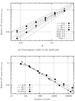
Accordingly to the above discussion, we chooseǫ=αHβ, β <1, and accordingly h=H3/2−β/2. With the above notation this is obtained when choosingM =α3/223β/2−1/2N3/2−3β/2. Thea prioriorder of convergence in H for the H1(Ω)-norm error is given by 1−β/3. An overview of different cases applied on the solution of problem (34) is reported in Table 2. In the last column of the latter we report the numerically obtained order in H. In Figure 6(a) we illustrate the concluding convergence behavior in the mesh-size graphically.
α β ǫ h M CO1 CO2
0.25 0 0.25 H3/2 N3/2/27/2 1 0.93 1 1/3 H1/3 H4/3 N 8/9≈0.89 0.79 1 2/3 H2/3 H7/6 N1/2√2 7/9≈0.78 0.74
no patch 2/3≈0.67 0.63
Table 2. Synoptic table of chosen patches and H1(Ω)-norm convergence orders (CO1 = a
priori order inH, CO2 = order obtained by numerical experience).
slope 1 slope 8/9 slope 7/9 slope 2/3no patch
ǫ=H2/3
ǫǫ== 0.25H1/3
H
R
el
a
ti
v
e
H
1-n
o
rm
er
ro
r
eH
h
0.1 0.01
0.1
0.01
(a) Convergence order in the mesh size.
no patch
ǫ=H2/3
ǫǫ== 0.25H1/3
Number of nodes
R
el
a
ti
v
e
H
1-n
o
rm
er
ro
r
eH
h
100000 10000
1000 100
10 0.1
0.01
(b) Error reduction vs. number of nodes.
Figure 11. Convergence ofuHresp. uHhtouwith respect to the mesh sizeHand the number of nodes.
4.
Application to glacier modeling
The basic continuum mechanics equation for mass conservation, momentum conservation and constitutive re-lation for such an ice flow have been studied by Fowler and Larson [9], Hutter [18] and Morland [19]. We are going to use in this work a model by Blatter [2], and for numerical studies consider a 2D vertical cut of the Gries glacier (Switzerland) in the direction of the motion of a glacier and horizontal invariance (the glacier is very large), as studied by Reist [21]. The model we use allows to simulate the horizontal velocity field of the ice mass and the effective stress. Changes in the basal surface, the interface between the ice mass and the rock bed, imply different conditions for the flow. We suppose that boundary conditions can change from free sliding to prescribed velocity, and reverse, along the basis. This directly relates to the solution for the velocity and thus for the stress field which is more or less regular. A good precision is necessary as the change from Neumann to Dirichlet conditions reflects non-locally in variations all over the ice mass.
4.1.
A mathematical model of a glacier.
The geometry of the 2D vertical cut of the ice mass is defined by the upper free surfaceSgiven byz=S(x),
x∈[a;b], which is supposed regular (i.e. no overhanging), and the basal surfaceBgiven byz=B(x),x∈[a;b], in cartesian coordinates (x, z) with thez-axis pointing opposite the direction of gravity. We call ΓS the upper surface of the glacier given by the points (x, z) such thatz=S(x) and ΓB the mountain base, the points (x, z) such thatz =B(x). We suppose that B(x)≤S(x) and denote by Ω the glacier domain occupied by ice, the set of points (x, z) such thatB(x)≤z≤S(x),x∈[a;b]. Furthermore we split ΓB in two parts ΓB,D where we consider the glacier fixed on the mountain, i.e. homogeneous Dirichlet boundary conditions for the velocity field, and ΓB,N where we consider Neumann boundary conditions for the velocity which represent a slip condition.
The model by Blatter [2] rewritten by Wagner in [22, Chapter 4] leads to the following problem: Find the horizontal velocityudefined in Ω such that
−div(µ(|∇u|)∇u) =f in Ω,
∂u
∂n = 0 on ΓS,
∂u
∂n = 0 on ΓB,N,
u= 0 on ΓB,D,
(35)
wheref =−14ρg ∂S
∂x, ρbeing the density of ice andg the acceleration of gravity, andµ=µ(s) is given by
A [µ(s)]n−1sn−1+σ0n−1
= 1
2µ(s), (36)
with A and σ0 constants, and n≥1 an exponent. In [13, Lemma 1] it is proven that µ as a function ofs is well defined by relation (36). We observe that for n= 1, µ(s) = 1/4A, and forn= 2, µ is readily explicited,
µ(s) =−Aσ0+
p
A2σ2 0+ 2As
/2As.
The horizontal velocity fielduis given by the above problem (35). Furthermore the effective stress fieldσ(II) is expressed through
σ(II)=µ(|∇u|)|∇u|. (37)
We will compute the velocity field of the glacier by solving numerically problem (35). We will use a finite element method, using a computational mesh adapted to the geometry of the problem.
4.2.
Weak formulation.
We establish a weak formulation of problem (35). By multiplying the first equation of the latter system by
ϕ vanishing on ΓB,D, by integrating by part on Ω and taking into account the natural boundary conditions (second and third equation of (35)) on ΓS and ΓB,N, by setting
aµ(u, ϕ) =
Z
Ω
we obtain
aµ(u, ϕ) =
Z
Ω
f ϕdΩ. (39)
Remark that aµ(u, ϕ) is linear with respect to ϕ, but nonlinear with respect tou becauseµ depends onu. Let nowV be the Banach space, V ={ϕ∈W1,p(Ω) :ϕ= 0 on ΓB,D}, where p= n+1n , with nthe exponent appearing in the flow law (36). In [13] it is proven that there existc1, c2>0 such that
c1(1 +|∇u|) 1
n−1≤µ(|∇u|)≤c
2(1 +|∇u|) 1
n−1, ∀|∇u| ∈(0; +∞), (40)
and hence µ(|∇u|)∇u∈Lq(Ω) with 1 p+
1
q = 1 (q =n+ 1), when u∈V. Consequently, the form (38) makes sense when u, ϕ∈V.
It follows that the weak formulation of problem (35) with natural boundary conditions on the upper surface ΓS and the part ΓB,N of the basal surface, and Dirichlet conditions on the part ΓB,D of the basal surface, is:
Find u∈V such that
aµ(u, ϕ) =
Z
Ω
f ϕdΩ, ∀ϕ∈V. (41)
Colinge and Rappaz prove in [7, Theorem 1] the uniqueness of the solution in the case of Dirichlet boundary conditions on all∂Ω. This result can be extended to our case of problem (41) with mixed Dirichlet-Neumann conditions.
4.3.
Discretization.
We discretize problem (41) by using hat functions. First we choose the mesh size H and consider an approximation of Ω by a polygonal domain which is still denoted by Ω with sides of length H. We denote by TH a regular triangulation of Ω with triangles K ∈ TH such that ∀K ∈ TH, diam(K)≤H. We assume that for each triangle K ∈ TH, K∩ΓB,N is either void or a side of K or a vertex of K, where ΓB,N denotes the polygonal line of∂Ω joining the fixed pointsAandB (see Figure 12). We introduceVH ={ψ∈ C0(Ω) :ψ|K ∈ P1(K),∀K ∈ TH andψ = 0 on ΓB,D}, where ΓB,D denotes the part of∂Ω corresponding to the part of the basal surface with Dirichlet boundary conditions, and call µH =µ(|∇uH|). We consider the following discrete problem: Find uH ∈VH such that
aµH(uH, ϕH) = Z
Ω
f ϕH dΩ, ∀ϕH∈VH. (42)
4.4.
Linearization.
In order to solve numerically the discrete variational problem (42) we use Picard’s iterative method. We apply the following steps:
• Initialization: SetuH,0 the solution of (42) withn= 1, i.e. µ=µH = 1/4A. • Fork= 1,2,3, . . . solve the following linear problem: Find uH,k∈VH satisfying
aµH,k−1(uH,k, ϕH) =
Z
Ω
f ϕH dΩ, ∀ϕH∈VH, (43)
whereµH,k−1=µ(|∇uH,k−1|).
A
B
u = 0
u = 0
du /dn = 0
du /dn = 0
Figure 12. Geometry, boundary conditions and triangulation (N = 50) of the Gries glacier. Grid constellation and illustration of two patches (M = 4,H/h= 4) around the pointsAand
B.
4.5.
Numerical illustration.
We illustrate our numerical model for a two-dimensional glacier on a vertical section along a flow line passing through the center of Gries glacier (Wallis, Swiss Alps). As the Gries glacier is large in the transverse direction our two-dimensional computations are relevant. The shape of the glacier [21] and the basic meshing withN = 50 intervals in thex-direction (and accordingly discretized in the z-direction to obtain a regular triangulation) is illustrated in Figure 12.
We study the nonlinear case with n = 2. For defining the right-hand side f, defined in (4.1), we set
ρg= 900·9.81·10−5and in the flow law (36) we takeA= 0.08 andσ
0= 0.1, as suggested by [21] and converted from the S.I. unit values from Greve [14, p. 936].
We use the relativeL2-discrepancy of the stress field as stopping criteria for the iterations due to linearization. When running the algorithm described in the Introduction (with a discrepancy of 10−3 in the corrections), we note that about 10 iterations are required to obtain convergence. We have implemented the model with the softwareFreefem++[17].
4.6.
Stress field on the mountain base.
Let us now turn to the stress field of the glacier and consider the nonlinear case. Before studying how to increase the precision on the approximation of the latter, we briefly outline its behavior along the mountain base, i.e. the boundary ΓB. Our knowledge of the behavior of the velocity field in the case of the (linear) Poisson problem with changing Dirichlet-Neumann boundary conditions (Section 2), and the result (40) meaning that
N= 800 NN= 200= 50
B A
ΓB
E
ff
ec
ti
v
e
st
re
ss
σ(I
I
)
50
40
30
20
10
0
Figure 13. Behavior of the stress fieldσ(II)(uH) on ΓBin the nonlinear casen= 2. Numerical values are not scaled to physical units. The Figure merely illustrates the relative behavior for differentN.
4.7.
Patches and precision of the glacier stress field
We consider in this section the stress field of the glacier and consider the application of patches. We show that the application of patches is efficient for reducing the error around the points of changing boundary conditions on the basal surface.
The study of the effective stress field (Figure 13) shows that the stress field blows up around the points of the boundary where the boundary conditions change.
With (37),σ(II) =µ(|∇u|)|∇u|, and (40), the minimal regularity requirement on the velocity fieldu∈V a subset ofW1,p(Ω) with p= (n+ 1)/n, suffices to haveσ
(II)∈L1+n(Ω), i.e. at leastL2(Ω), sincen≥1. Hence the stress field isL2-integrable, and theL2-norm is adapted to measure it.
In our model, the boundary of the glacier domain Ω has two points A and B on the basal surface where it presents a Dirichlet-Neumann change in the boundary conditions (see Figure 12). Furthermore, we apply different patches with (M + 1)(M/2 + 1) discretization points in the regions aroundA andB in order to see how to sharpen the results.
We consider two types of patches as in Section 2. A first type, called fixed patch ΛA, ΛB, which in the original mesh with N = 50 points covers exactly one triangle in all directions aroundA andB, and a second type which covers, at any refinement level, one triangle in all directions: it is what we call a variable patch. An illustration of fixed patches and their size for the refined mesh with N = 50 and M = 4, i.e. H/h= 4, is depicted in Figure 12. For the triangulations of ΛAand ΛB, we consider refinements such that the diameterh
of the fine triangulation ish=H/2,H/4 orH/8.
As mentioned previously, about 10 iterations are necessary to cope with the iterative method for the linearized problem. Currently, we have an inside loop corresponding to the iterations of the correction algorithm. Requiring the relative discrepancy of the velocity field in theL2-norm to be below 10−2, the inner-loop convergence needs 2 to 3 full iterations.
We measure the L2-norm relative error (n = 2) of the stress field σ
Hh = σ(II)(uHh) with respect to the “almost exact” solutionu given byuH with N = 3200 andσ=σ(II)(u). We evaluate the norms in domains ΛAand ΛB for N = 50 and 100, and for situations without patch and with patch. For the situation where we apply a patch we consider either two fixed patches or two variable patches (smaller forN = 100) aroundAand
N M ||σ−σHh||L2(ΛA)
||σ||L2(Λ
A)
||σ−σHh||L2(ΛB)
||σ||L2(Λ
B)
50 – no patch 0.264 0.310
2 H/h= 2 0.194 0.237
4 H/h= 4 0.168 0.170
8 H/h= 8 0.184 0.155
Fixed patch, large region
100 – no patch 0.201 0.215
4 H/h= 2 0.171 0.134
8 H/h= 4 0.181 0.120
16 H/h= 8 0.164 0.111
Variable patch, small region
100 – no patch 0.265 0.290
2 H/h= 2 0.225 0.220
4 H/h= 4 0.239 0.155
8 H/h= 8 0.232 0.193
Table 3. L2-norm relative error of the velocity and the stress fields in the patches (withn= 2).
Considering the data reported in Table 3, we note that the reduction of the error is efficient. If we evaluate the errors in variable regions, though refining the grids by a factor 2, fromN = 50 to 100 with no patch for example, we note no considerable change in the value of the error as the domain for evaluation has in the same time tightened around the point of singular behavior.
We conclude with a precision gain for the stress field due to the application of patches. Taking for example the caseN = 50 with no patch and a patch withM = 8 aroundB, we report that the error on the stress field is divided by two! Furthermore, we can also compare the convincing pair of situations ofN = 50 with a patch (M = 4 or 8) and of N = 100 with no patch. While using much less discretization points, applying a small, well chosen patch yields better results than a global refinement.
Finally, the question of the optimal size of the patch arises. To give an answer to this point, we consider the coarse discretization with N = 50 and consider the relativeL2(Ω)-norm error of the effective stress field with respect to the above introduced “almost exact” solution.
Without any patch, this error yields 0.153. Applying patches around A and B with the size as shown in Figure 12 (i.e. covering one coarse triangle in each direction around the point A or B, the patch is large by 2H) and a ratioH/h= 2, we reduce the error and get 0.121.
If we want to further improve the solution, we can either enlarge the regions over which we consider the patches, or refine the chosen patches. Refining the patches such thatH/h= 8, reduces the error to the value 0.110. However applying patches around A and B that are 8H large (four times larger, four times higher), keeping the ratio H/h = 2 constant, the relative error does not improve: 0.126. This means that in this particular situation, the size of the patch is accurately chosen small, covering the region where the solution varies most.
In conclusion, note that the correction method and an accurate analysis for the placement of the patches pays out most when we consider evolution problems (e.g. the modeling of glaciers as done by Reist [21]).
Acknowlegements
References
[1] I. Babuska. Finite element method for domains with corners.Computing (Arch. Elektron. Rechnen), 6:264–273, 1970. [2] H. Blatter. Velocity and Stress Fields in Grounded Glaciers: A Simple Algorithm for Including Deviatoric Stress Gradients.
J. Glac., 41(138):333–344, 1995.
[3] M. Bourlard, M. Dauge, and S. Nicaise. Error estimates on the coefficients obtained by the singular function method.Numer. Funct. Anal. Optim., 10(11-12):1077–1113 (1990), 1989.
[4] S.C. Brenner. Multigrid methods for the computation of singular solutions and stress intensity factors i: corner corner singu-larities.Math. Comp., 68(226):559–583, 1999.
[5] Z. Cai and S. Kim. A finite element method using singular functions for the Poisson equation: corner singularities.SIAM J. Numer. Anal., 39:286–299, 2001.
[6] P.G. Ciarlet. Basic error estimates for elliptic problems. In P.G. Ciarlet and J.L. Lions, editors,Finite Element Methods (Part 1), volume II ofHandbook of Numerical Analysis, pages 17–351. North-Holland, 1991.
[7] J. Colinge and J. Rappaz. A Strongly Nonlinear Problem Arising in Glaciology.M2AN, 33(2):395–406, 1999.
[8] M. Dauge.Elliptic boundary value problems on corner domains, volume 1341 ofLecture Notes in Mathematics. Springer, 1988. [9] A.C. Fowler and D.A. Larson. On the flow of polythermal glaciers. I. Model and preliminary analysis.Proc. R. Soc. London,
Ser. A, 363:217–242, 1978.
[10] J. Glen. The creep of polycrystalline ice.Proc. R. Soc. London, Ser. A, 228(1175):519–538, 1955.
[11] R. Glowinski, J. He, A. Lozinski, J. Rappaz, and J. Wagner. Finite element approximation of multi-scale elliptic problems using patches of elements.Numer. Math., 101(4):663–687, 2005.
[12] R. Glowinski, J. He, J. Rappaz, and J. Wagner. Approximation of multi-scale elliptic problems using patches of finite elements.
C. R. Acad. Sci. Paris, Ser. I, 337:679–684, 2003.
[13] R. Glowinski and J. Rappaz. Approximation of a Nonlinear Elliptic Problem in a Non-Newtonian Fluid Flow Model in Glaciology.M2AN, 37(1):175–186, 2003.
[14] R. Greve. A continuum-mechanical formulation for shallow polythermal ice sheets.Phil. Trans. R. Soc. Lond., Ser. A, 355:921– 974, 1997.
[15] P. Grisvard.Elliptic Problems in Nonsmooth Domains, volume 24 ofMonographs and Studies in Mathematics. Pitman, 1985. [16] P. Grisvard.Singularities in Boundary Value Problems, volume 22 ofResearch Notes in Applied Mathematics. Masson, 1992. [17] F. Hecht, O. Pironneau, and K. Ohtsuka.Freefem++.http://www.freefem.org.
[18] K. Hutter. Theoretical Glaciology: Material Science of Ice and the Mechanics of Glaciers and Ice Sheets. Mathematical Approaches to Geophysics. D. Reidel Publishing Company / Terra Scientific Publishing Company, 1983.
[19] L.W. Morland. Thermo-mechanical balances of ice sheet flows.Geophys. Astrophys. Fluid Dyn., 29:237–266, 1984.
[20] G. Raugel. R´esolution num´erique par une m´ethode d’´el´ements finis du probl`eme de Dirichlet pour le laplacien dans un polygone.
C. R. Acad. Sci. Paris, Ser. A, 286:791–794, 1978.
[21] A. Reist.Mathematical analysis and numerical simulation of the motion of a glacier. PhD thesis, EPFL, Lausanne, Switzerland, 2005.