Identifying, Mapping, and Exploring Excess Relationships in Engineered Systems Relevant to Service Phase Evolution

ABSTRACT

CANSLER, ETHAN ZACHARIAH. Identifying, Mapping, and Exploring Excess Relationships in Engineered Systems Relevant to Service Phase Evolution. (Under the direction of Dr. Scott Ferguson).

i Identifying, Mapping, and Exploring Excess Relationships in Engineered Systems

Relevant to Service Phase Evolution

by

Ethan Zachariah Cansler

A thesis submitted to the Graduate Faculty of North Carolina State University

in partial fulfillment of the requirements for the degree of

Master of Science

Aerospace Engineering

Raleigh, North Carolina 2015

APPROVED BY:

_______________________________ Dr. Scott Ferguson

Committee Chair

________________________________ ________________________________

ii BIOGRAPHY

iii ACKNOWLEDGMENTS

iv TABLE OF CONTENTS

LIST OF TABLES ... vi

LIST OF FIGURES ... vii

Introduction ... 1

Evolvability ... 1

Nature and Origins of Excess ... 3

Motivation ... 4

Background ... 8

System Evolvability and Excess ... 8

Change Relationships between Components ... 9

Design Structure Matrices... 9

Change Propagation ... 11

Functional Modeling ... 12

Real Options Theory ... 14

Conclusions from Literature Review ... 14

Foundational Theory ... 16

Categorizing Excess ... 16

Excess Basis ... 18

Resolution of Excess Flows ... 22

Developing a Mapping Approach for System Excess... 23

Step 1: Collect Stakeholder Specifications ... 25

Step 2: Identify System Architecture and Relationships ... 26

Step 3: Assemble Excess Map ... 38

Step 4: Identify State Parameters ... 40

Evaluating System Level Excess ... 41

Map Quality and Criteria for Update ... 43

Case Study 1 Conclusion: Heat Gun Evolution Examples ... 43

Heat Gun Evolution 1: Replace Tri-Mode Switch with Variable Voltage Switch ... 43

Heat Gun Evolution 2: Increase Output Temperature to 750 °C ... 44

Case Study 2: Coffee Maker ... 44

v

Coffee Maker Evolution Examples ... 57

Scalability Case Study ... 59

Subsystem 1: Engine ... 61

Subsystem 2: Transmission... 62

Subsystem 3: Cutting Attachment ... 63

String Trimmer Excess Map ... 64

Stress Test Approach... 67

Stress Testing in Engineering ... 67

Stress Test Approach Steps ... 68

Step 1: Collect Future Needs and Specifications ... 68

Step 2: Generate Solutions ... 69

Step 3: Evaluate Impacts ... 70

Step 4: Judge Fitness/Review Excess Placement... 71

Stress Test Case Study Preliminaries ... 71

Toy Dart Gun Excess Map Creation ... 72

Stress Test Case Study ... 86

Step 1: Collect Future Needs and Specifications ... 86

Steps 2 and 3: Generate Solutions and Evaluate Impacts ... 87

Step 3 Continued: Review Overlapping Future Needs ... 97

Step 4: Judge Fitness/Review Excess Placement... 99

Conclusions and Future Work ... 103

Research Question 1: How can excesses pertinent to service phase evolution be identified in a general system? ... 103

Research Question 2: How can designers relate the identified excesses to the system’s ability to meet future needs? ... 104

Opportunities for Future Work ... 105

REFERENCES ... 106

vi LIST OF TABLES

Table 3.1: Excess Basis... 19

Table 3.2: Structural Excess Optional State Parameters ... 20

Table 4.1: Heat Gun Component Excesses ... 39

Table 4.2: Coffee Maker Component Excesses ... 55

Table 4.3: String Trimmer Needs and Specifications ... 60

Table 5.1: Dart Gun Component Measurements ... 72

Table 5.2: Dart Gun Component Excesses ... 85

Table 5.3: Overlapping Future Needs ... 97

vii LIST OF FIGURES

Figure 2.1: Sample HD-DSM Faces for Heat Gun ... 11

Figure 2.2: Portion of Heat Gun Functional Diagram ... 13

Figure 3.1: Compatibility and Functional Flows ... 18

Figure 3.2: Naming Scheme for Excess Types ... 19

Figure 4.1: Excess Mapping Procedure ... 24

Figure 4.2: Heat Gun [42] ... 24

Figure 4.3: Variable Level of Abstraction ... 27

Figure 4.4: Excess Map Segment for General Architecture ... 28

Figure 4.5: Disassembled Heat Gun ... 30

Figure 4.6: Heat Gun Case ... 30

Figure 4.7: Case Excess Map Contribution ... 32

Figure 4.8: Cord Excess Map Contribution ... 32

Figure 4.9: Heat Gun Switch ... 33

Figure 4.10: Switch Excess Map Contribution ... 34

Figure 4.11: Heat Gun Heating Coils ... 34

Figure 4.12: Heating Coils Excess Map Contribution ... 35

Figure 4.13: Heat Gun Fan... 36

Figure 4.14: Fan Excess Map Contribution ... 37

Figure 4.15: Heat Gun Nozzle ... 37

Figure 4.16: Nozzle Excess Map Contribution ... 38

Figure 4.17: Heat Gun Excess Map ... 41

Figure 4.18: Coffee Maker [53] ... 45

Figure 4.19: Coffee Maker Body ... 47

Figure 4.20: Body Excess Map Contribution ... 48

Figure 4.21: Cord Excess Map Contribution ... 49

Figure 4.22: Coffee Maker Switch ... 49

Figure 4.23: Switch Excess Map Contribution ... 49

Figure 4.24: Coffee Maker Heating Element ... 50

Figure 4.25: Heating Element Excess Map Contribution ... 51

Figure 4.26: Coffee Maker Brew Basket ... 52

Figure 4.27: Brew Basket Excess Map Contribution... 52

Figure 4.28: Coffee Maker Hot Plate ... 53

Figure 4.29: Hot Plate Excess Map Contribution ... 53

Figure 4.30: Coffee Maker Carafe ... 54

Figure 4.31: Carafe Excess Map Contribution ... 54

Figure 4.32: Coffee Maker Excess Map ... 56

Figure 4.33: String Trimmer [57] ... 60

Figure 4.34: Engine Excess Map ... 62

Figure 4.35: Transmission Excess Map ... 63

Figure 4.36: Cutting Attachment Excess Map ... 64

viii

Figure 5.1: Stress Test Approach Flowchart... 68

Figure 5.2: Toy Dart Gun [62] ... 71

Figure 5.3: Dart Kinetic Energy Required vs. Distance for Level Fire at 1m ... 73

Figure 5.4: Dart Gun Body ... 75

Figure 5.5: Dart Gun Component Layout ... 75

Figure 5.6: Body Excess Map Contribution ... 76

Figure 5.7: Dart Gun Slide Grip ... 76

Figure 5.8: Slide Grip Excess Map Contribution... 77

Figure 5.9: Dart Gun Slide Pump ... 77

Figure 5.10: Slide Pump Excess Map Contribution... 78

Figure 5.11: Dart Gun Flex Tube ... 78

Figure 5.12: Flex Tube Excess Map Contribution ... 78

Figure 5.13: Dart Gun Check Valve/Release ... 79

Figure 5.14: Check Valve/Release Excess Map Contribution ... 79

Figure 5.15: Dart Gun Charge Pressure Vessel ... 80

Figure 5.16: Charge Pressure Vessel Excess Map Contribution ... 80

Figure 5.17: Dart Gun Floating Pressure Seal ... 81

Figure 5.18: Floating Pressure Seal Excess Map Contribution ... 82

Figure 5.19: Dart Gun Rotary Barrel ... 82

Figure 5.20: Rotary Barrel Excess Map Contribution ... 83

Figure 5.21: Dart Gun Trigger/Advance Assembly ... 83

Figure 5.22: Trigger/Advance Assembly Excess Map Contribution ... 84

Figure 5.23: Dart Gun Ratchet Shaft ... 84

Figure 5.24: Ratchet Shaft Excess Map Contribution ... 84

Figure 5.25: Toy Dart Gun Excess Map ... 86

1 Introduction

Designs are created in response to market opportunities that are driven by the identification of customer needs. As the design process advances, needs are mapped to numerical specifications, which are in turn translated to a system architecture [1]. However, the environment in which a system operates, and the needs that it is responsible for satisfying, may change over the service life of the system. Changes to initial needs, or the identification of new needs, after the design has been fielded are hereafter referred to as ‘future needs’.

Evolvability

The B-52 is one system that has successfully been able to respond to future needs. Originally designed and deployed as a long-range nuclear strike bomber in 1955, it is expected to serve until at least the 2040s [2]. Between its original introduction and now, the role of the B-52 has shifted from a high altitude nuclear strike bomber, to a low altitude conventional bomber, to a platform for standoff weapons [3]. The ability to take on these role changes were enabled by the payload capacity associated with the airframe, the ability to expand the payload volume via the ‘big belly’ modification, and reinforcing the interface structure between wings and fuselage [4].

In contrast, the F/A-18 is a system that has failed to meet future needs. The F/A-18 was originally introduced in 1983 as a joint attack and air superiority fighter. Over time the needs that the system faced changed due to developing technologies. These needs included the ability to return unused smart weapons to the carrier rather than dropping them at sea unused (thereby placing additional load on the landing structures) and the requirement to accommodate a greater volume of electronic warfare equipment. An updated version of the plane deployed in 1995 was redesigned so thoroughly that there is only 10% commonality between the original and new airframes [5]. Such a drastic redesign indicates that the original system was not capable of evolving to meet future needs due to factors including insufficient structural capacity of the landing gear and insufficient volume available within the fuselage.

2 value when faced with future needs is made possible by service phase evolution – formally defined as the ability of a system to physically transform from one configuration to a more desirable configuration while in service. The motivation for evolvability research is based on the belief that systems capable of service phase evolution possess greater value over their lifespan than those that are not [6].

Other approaches in the literature to ensure that a system is capable of meeting future needs include reconfigurability [7] and robustness [8]. However, these approaches have shortcomings, particularly for systems that are expected to be in service for a significant amount of time. Implementing reconfigurability is a choice made in the design phase that explicitly allows aspects of the system to assume a range of configurations. These configurations can be a set of fixed points or a bounded range on a continuum. Airfoils that incorporate flaps and/or slats to change the wing’s flight characteristics is an example of reconfigurable design.

Robust system design seeks to make a system insensitive to variations in its operating environment, without any alteration to the system while in service – a valid approach, but one that expends more resources than would be necessary if the system could be strategically changed. However, achieving robustness is often accomplished by sacrificing system performance. This is done by finding a location in the design space where the objective function contours are relatively flat. Such a location in the design space is often not co-located with the design that maximizes or minimizes system performance. Further, as the projected system lifespan is increased, the envelope of uncertainty is also expanded, meaning that applying robust design theory to a system with a long projected service life and completely unknown future needs would result in a drastically over-built (or under-performing) system.

3 Nature and Origins of Excess

Excess is defined as surplus in a system or component beyond what is currently required of it [9]. These potential surpluses occur in inter-component relationships, or relationships between components and the external environment. Much like enthalpy and entropy in thermodynamics, there is no such thing as ‘absolute excess’. Rather, excess is a relative measurement of the difference between the capabilities of the designed system and design specifications. These relationships fall into one of three categories: flow (transmitted energy, signal, or material), structural (stress or strain) or geometric (occupied length, area, or volume).

In practical engineering terms, excess occurs in situations such as:

 wiring carrying only 7 A of current when rated with an ampacity of 10 A,  a pressure vessel operating at 200 MPa when it is certified for 400 MPa,  an equipment room holding 20 m3 of hardware when it can contain 35 m3.

The surplus embodied by the Factor of Safety (FoS) is generally considered to be independent from the excesses used for system evolvability. As an example, consider a structure made of material with a yield strength of 300 MPa. With a FoS of 3, the usable material strength is 100 MPa. If subjected to a design load that produces stress of 70 MPa, the excess within the structure is 30 MPa. The only situation where part of the FoS for a system may be converted to usable excess occurs when the FoS has been revised downward due to either overly conservative initial estimates or a less severe operating environment than originally planned.

4 and non-load-bearing walls for the sake of easier construction, even though for the latter application their full strength is unnecessary.

Since designers are incapable of knowing the future, the excess that is originally designed into the system may not be constant over time. Rather, the excess present in a systems may vary due to system evolutions or changes in system specifications while in service. When, lower than anticipated service requirements are realized, excesses are created in the components that are consequently underutilized.

Motivation

The formulation shown in Equation 1.1 was developed in [9] and refined in [10]. Here, evolvability E is expressed as a function of excess X, evolvability gain per unit excess gx, and

the upper and lower bounds of usable excess xl and xu. Excess and its upper and lower usable

bounds have the unit of percent (%) of the normalized design quantity that is being measured, while the gain per unit excess has units of reciprocal percent (1/%). Two classes of US Navy aircraft carrier – the Nimitz class and the Ford class – were compared based on four parameters: displacement, volume, stability, and electrical power. These parameters were sourced from the decades of empirical design experience reflected in [11] [12]. It was found that the Nimitz class aircraft carrier had an evolvability of 19.2 yr-%, while the Ford class carrier had an evolvability of 257 yr-%. These units resulted from the fact that the US Navy measures aircraft carrier evolvability in hypothetical years of extended service life. When using Equation 1.1, the numbers that are produced have meaning when they are compared, as they represent the relative evolvability of different design options for a single system. Hence, the Ford class was demonstrated to be significantly more evolvable than the Nimitz class.

𝐸 = ∫ 𝑋 ∙ 𝑔_𝑥 𝑑𝑋

𝑥𝑢

𝑥𝑙

( 1.1 )

5 parameters such as power generation to low-level parameters such as tensile strength of the screws affixing speakers to bulkheads. The demonstrative case study in [9], comparing two classes of US Navy aircraft carrier, benefited from decades of empirical knowledge that told designers which excesses were important to enable service phase evolvability. Practically speaking, such knowledge allows designers to embed suitable quantities of these excesses in the system. Clearly, a subset of the possible excesses that can be described for a system are sufficient to describe a system’s evolvability; however, the question remains of how to identify such excesses for general systems that do not necessarily benefit from prior experience.

Another consideration driving selection of excesses is that they must be of the correct type, quantity, form, and location to be usable in bringing about system change [13]. This means that for an evolution to occur, there must be the right kind of excess in every affected component, there must be enough of it, it must be of the right form, and it must be accessible to the component that requires it to undergo the evolution. As a simplified practical example, an evolution to a building might require placing a new piece of equipment in a specific location. However, the evolution may only proceed if there is sufficient volume, energy, and load-carrying capacity at said location within the building, if these excesses are collocated with the intended equipment placement, and if these excesses are of the correct form – i.e. the excess volume is in a shape that can accept the new equipment, the energy is electrical and of the correct voltage and/or frequency, and the load-carrying capacity of the structural members can be interfaced with the new equipment.

Therefore, the question remains of how to identify excesses within general systems that are relevant to system evolvability. This leads to the first research question explored in this thesis:

Research Question 1:

How can the presence and quantity of excess pertinent to service phase evolution be identified?

6 deck railings is highly unlikely to have an impact on the ability of the ship to evolve. It is not hard to categorize those two excesses as relevant and irrelevant, respectively, because they are extreme examples. However, exactly where to draw the line between relevant and irrelevant excesses is not clear.

Designers are incapable of knowing with certainty the future needs a system will face. When considering system evolvability, a simplifying assumption used in [10] was that the top level functions of a system remain fixed. In simple terms, this means that an aircraft carrier will always transport and launch aircraft and a coffee maker will always brew coffee. This assumption could be used to reduce the scope of excesses considered for their contribution to evolvability to those that contribute to the current functions of the system, as future functions would be related.

As excess is consumed to meet future needs, deliberate placement of excess in a system must be a function of unknowable future needs. Blindly adding excess to components or subsystems (even if they are the excesses identified as pertinent to system evolvability) adds cost without guaranteed benefit, leading to decreased system value. These considerations lead to the second research question:

Research Question 2:

How can designers relate the quantities of the identified excesses to the system’s ability to meet future needs?

There is limited discussion in the literature regarding the inclusion of excess to meet future needs. The available literature generally describes situations where designers draw on past experience designing similar systems, as in [11] [12]. However, there is a lack of guidance for systems without the benefit of empirical design knowledge.

7 quantities, diminish the evolvability of the design and reduce the utility of other excesses. Therefore, the idea that a system design can be stress tested to find ‘bottlenecks’ for system evolution is investigated. Beyond identifying locations in which excess should be added, the similar idea of revealing excesses that are superfluous, i.e. those that support system changes surpassing those enabled by the other excesses, is explored.

8 Background

No analytical method exists in the literature with the ability to map or quantify excess for an engineered system. Yet, it is recognized that system evolvability is intrinsically tied to engineering change. Exploring how to manage change within an engineered system is a topic that has received significant attention in the literature. This chapter discusses research introducing the concept of excess, explores methods of modeling a system, and characterizes how changes propagate.

System Evolvability and Excess

The last few years of evolvability-focused design research have seen a progression from design guidelines to mathematical formulations. Work in [14] [15], for example, introduced empirically-derived design guidelines to enable future evolvability. These guidelines are centered around:

 system modularity,  scalability,

 reduction of unnecessary parts,  decoupling interfaces,

 maintaining clearances and usable area,  designing tunable components,

 and providing energy storage/importation capabilities in excess of the original requirements.

9 should be assigned to impact the successful completion of the original design rather than how they might lead to system evolvability.

Moving toward a more mathematical framework, Tackett et al. [9] introduced excess as a variable controlled by designers, meaning that they had control over the amount of surplus present in each component of a system. Further work developed a mathematical formulation of system evolvability as a function of excess [10] as was shown in Equation 1.1. This work investigated excess in two classes of naval aircraft carriers, the older Nimitz class and the upcoming Ford class. The Ford class was estimated to be more evolvable that the Nimitz class when considering an upgrade from traditional steam catapults to electromagnetic catapults for launching aircraft. A limitation of this work, however, was that it benefited from empirical knowledge of naval design experts that defined the types of excess within a system and how evolvability was tied into service life [11] [12].

Change Relationships between Components

Quantifying the excess within a system is necessary if it is to eventually be used as a parameter when designing for evolvability. A specific target of the literature review was strategies that integrate numerical information about components associated with change. ‘Engineering change’ has been defined as occurring while the system is still being designed, and is defined as “an alteration to parts, drawings, or software that have already been released during the product design process. The change can be of any size or type; the change can involve any number of people and take any length of time.” [18]. Service phase evolution is by definition different from engineering change, as it occurs after the system has been constructed and deployed. However, system evolution requires redesign, and works exploring engineering change may be applicable when predicting the ability of a system to evolve.

Design Structure Matrices

10 or task while the rows represent the affected component or task. The information content of DSMs has been expanded to include additional detail about component relationships. Pimmler and Eppinger [21], for example, defined four classes of interaction: Spatial, Energy, Information and Material. Sosa et al. [22] added a fifth class of interaction, Structural. With these five classes, all relationships between components could be described. However, the presence of five different interaction types on a two-dimensional plot led to challenges of effectively conveying information.

In support of analyzing flexibility for future system evolvability, Tilstra et al. [23] developed the High-Definition Design Structure Matrix (HD-DSM) methodology to account for direct change propagation potential throughout a multi-domain engineered system. The HD-DSM methodology maps changes to the domain to which they correspond, significantly increasing resolution over the traditional DSM. It accomplishes this by making the DSM three-dimensional, such that each face applies to a particular domain. The domains are collected in an ‘Interaction Basis’ and are largely sourced from the functional basis defined by Hirtz et al. [24] but also correspond to those used in [21] [22]. The HD-DSM process reveals an interesting point: provided that two dimensions of the DSM structure correspond to originating and receiving components, the DSM structure can be extended to any number of dimensions.

11

1 2 3 4 5 6

Case - 1

Controller - 2

Fan Motor - 3

Heat Coils - 4

Wire - 5

Fasteners - 6

1 2 3 4 5 6

Case - 1

Controller - 2

Fan Motor - 3

Heat Coils - 4

Wire - 5

Fasteners - 6

1 2 3 4 5 6

Case - 1

Controller - 2

Fan Motor - 3

Heat Coils - 4

Wire - 5

Fasteners - 6

Electrical Energy Domain Gas Material Domain Thermal Energy Domain Figure 2.1: Sample HD-DSM Faces for Heat Gun

Change Propagation

A key segment of change research regards change propagation, which has been defined in the literature as “the process by which a change to one part or element of an existing system configuration or design results in one or more additional changes to the system, when those changes would not otherwise have been required” [25]. Clearly, change propagation is not desirable; ideally, a change to one component in a system design would never require change in another. Change propagation analysis has received increased attention in engineering design research because of the value associated with efficient change management in the system design process.

Eckert et al. [26], recognizing that some components will have a greater effect on system change than others, developed four classifications for components: constants, absorbers, carriers, and multipliers. Constants are unaffected by change and have no relationship with change whatsoever. Absorbers can absorb more changes than they cause and diminish change complexity. Carriers cause and absorb changes in roughly equal measure, and do not affect change complexity. Multipliers cause more changes than they absorb, and increase change complexity.

12 analysis, however. For example, Suh et al. [27] explored the use of quantified change propagation analysis to strategically embed product flexibility. Some forms of change propagation analysis target the overall risk to a design of change. Risk has been defined as the likelihood of a change times its impact on redesign (i.e. how much work must be redone) [28]. Tools have been developed to quantitatively describe risk, including the Change Propagation Method [29], RedesignIT [30], and a Matrix-Calculation-Based Algorithm [31].

Other researchers have sought to track changes over multiple domains; Pasqual and de Weck [32] developed a change propagation network that included information from the coupled product, change, and social domains. Over time, change propagation research has incorporated both more domains and numerical information to increase the resolution of the system change pathways being analyzed.

Change propagation analysis seeks to highlight sources of potential change to aid designers in minimizing its propagation. However, design for service-phase evolution mandates specific change(s) to specific component(s) and requires knowledge of physical component-specific parameters that change propagation analysis is generally not equipped to offer. Further, the presentation styles of change propagation analysis are typically not conducive to visualizing the impacts of a specific change or evolution throughout a system. To that end, other techniques from the literature were sought that are capable of representing an entire set of relationships between subunits of a system within a single view. The most promising candidate was functional modeling, as discussed next.

Functional Modeling

13 transmitting air from the atmosphere to the base of the dart (as propellant), and converting the aiming signal from the operator to a flight direction for the dart [33]. This approach allows a designer to consider what the system is intended to do. In an effort to standardize the nomenclature in a functional model, Hirtz et al. [24] developed a reconciled functional basis that addressed both the functional flows between components and the functional vocabulary pertaining to the individual components’ operations. The ability to abstract a system has allowed functional modeling to be used for a variety of tasks that extend beyond pure conceptual design. For example, Kalyanasundaram and Lewis [35] used the functional models of two systems as the first phase in determining which functional flows would be shared in a unified product. Kurtoglu and Tumer [36] have also employed a functional model as a tool for evaluating functional-failure risk in systems in the conceptual design phase.

As a reference, a selected portion of a traditional functional diagram for a heat gun is shown in Figure 2.2.

Import Human Signal

Actuate Electricity Import

Electricity

Convert Elec. To Thermal Hand

Hand

Energy Signal Material

Figure 2.2: Portion of Heat Gun Functional Diagram

14 While functional modeling is excellent for visualizing how flows of energy, signal, and mass travel through a system in terms of its functional blocks, there is no way to tell how these flows interact with the physical components of the system, nor are the flows quantified. Therefore, there are no provisions for the information that is needed when mapping excess – a physical architecture based set of quantified excess relationships (that include more factors than only flows of energy, signal, and mass).

Real Options Theory

Real options theory, originally used in the field of economics, has been adapted for use in engineering as described in [38]. A real option is the right, but not the obligation, to undertake a specific action. In the context of engineering, a real option is the ability to exercise a predetermined change to a deployed system, or in other words, a designed-in future evolution. Some works in the engineering literature [39] [40] have applied real options theory to the problem of maximizing system value when a finite set of future evolutions is known. However, the traditional formulation of real options analysis, reliant on a finite set of future needs, is incapable of analyzing systems with unknowable future needs.

Conclusions from Literature Review

15 a system. It carries the additional benefit of being a visually accessible and intuitive means of tracking component relationships throughout a system, unlike with HD-DSMs.

Regarding DSM-based methods, though their visual arrangement is not suitable to mapping excesses in a system, aspects of their approaches are useful for mapping excess flows within a system. HD-DSMs assimilate information from any necessary domain, while change propagation approaches incorporate numerical information regarding component relationships. Since excess can occur in any component relationship, an approach capable of interacting with any domain is necessary. To standardize the domains of excess considered, a formal set of excesses, similar to the HD-DSM interaction basis, is also needed.

16 Foundational Theory

The preceding chapter detailed approaches in the literature pertaining to change and system modeling and analysis. This section details the underlying theory particular to the nature and treatment of excesses for enabling system change, and serves as the foundation of the work developed in Chapters 4 and 5.

The approach presented in this thesis is based on the assumption that future needs placed on a system are unknown, but bounded. Specifically, bounded means that the functional purpose of a function chain does not change over time. Such an assumption is supported by examples studied in the prior work of [10], wherein the demands placed on aircraft carriers over time did not shift the core purpose (launching aircraft) but did change the means by which that purpose was achieved (electromagnetic versus steam-driven catapults).

Categorizing Excess

Designers often deliberately include some quantity of excess for reasons discussed in the four categories below. The first three categories - deterministic, epistemic, and aleatory - are differentiated by their associated uncertainties, while the fourth category, consequent, originates as a byproduct of other design decisions.

 Deterministic excess is concerned with the excess that is expected to be consumed over the course of the system’s lifetime based on original system requirements. A common example is the thickness of sacrificial plating that is expected to corrode in the service environment. Deterministic excess is assigned according to the environment that the system is expected to face and its designed service life.

 Epistemic excess is strategically placed within a design to address future needs that are not yet realized, but could reasonably occur during the system’s lifetime. When placing epistemic excess, designers might draw from sources such as institutional experience, expected technological trends, expected market trends, etc.

17 future need emerges in the course of the system’s service life. No method exists to guide the inclusion of aleatory excess.

 Consequent excess occurs as a result of the presence of standardized components within a design that exceed required capabilities. Examples include fasteners and commercial off the shelf components that are chosen to accommodate standardized sizing, commonality, or to minimize redesign. These excesses may not be of significant quantity but can still be utilized to meet future needs.

If component relationships are considered, flows between components can be divided into two categories (as shown in Figure 3.1):

 Compatibility flows occur in the relationships required for a component to function, and always are shown as input flows. For an electric motor, compatibility flows could include the electrical current that the motor draws, the volume that the motor occupies, the ability to withstand/convey the waste heat of the motor away, the reaction torque from the motor, and the support reaction required for the weight of the motor.

 Functional flows occur in the functional outputs of components. These either become compatibility flows for other components or are system outputs across the control volume. For an electric motor, functional flows could include the torque and/or power that the motor develops, depending on which is important for the motor’s particular application.

An implication of this classification scheme is that the indicated directionality of flow does not necessarily match that of the associated physical parameters. Rather, flow is always shown with the arrow pointing from the supplying component to the dependent component. An example of this behavior occurs when a component must dissipate a waste flow to operate. While the waste flow (of material, heat, etc.) is literally flowing away from the originating component, the arrow points from the component that dissipates the flow to the originating component. This is because the functionality of the originating component depends on the component that dissipates the waste flow.

18 consider an electric motor. If additional torque is required from the motor (one of its functional flows) it will require additional current (one of its compatibility flows). In contrast, as long as the same motor is used, the volume required to accommodate it (another of its compatibility flows) will not vary with the required torque. Critical to a system’s functionality is the ability of each component to satisfy the requirements of any connected components. The presence of sufficient excess in each contributing component permits change to the desired performance characteristics of the system.

Motor

Torque

Electrical Current

Compatibility Flows

Functional Flows Component

Figure 3.1: Compatibility and Functional Flows

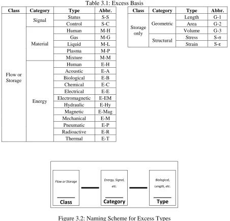
Excess Basis

19 Table 3.1: Excess Basis

Class Category Type Abbr. Class Category Type Abbr.

Flow or Storage

Signal Status S-S

Storage only

Geometric

Length G-1

Control S-C Area G-2

Material

Human M-H Volume G-3

Gas M-G

Structural Stress S-σ

Liquid M-L Strain S-ε

Plasma M-P Mixture M-M

Energy

Human E-H Acoustic E-A Biological E-B Chemical E-C Electrical E-E Electromagnetic E-EM

Hydraulic E-Hy Magnetic E-Mag Mechanical E-M

Pneumatic E-P Radioactive E-R Thermal E-T

Flow or Storage

Class

Energy, Signal, etc.

Category

Biological, Length, etc.

Type

Figure 3.2: Naming Scheme for Excess Types

20 The second categorical extension is Structural, with associated type entries of stress (σ) and strain (ε). Structural excess occurs when an artifact could withstand a greater stress or strain than currently required. Component-level structural excesses may be consumed by other components within a system or by conditions imposed by the operating environment.

When describing structural parameters of components, the true excesses that are being consumed are stress and strain. However, designers may find it more convenient for certain applications to define state parameters such as Load, Pressure, and Torque to describe the structural excess relationships between components, with the understanding that such state parameters ultimately map back to the stress and strain characteristics of the materials. In view of these factors, the supplementary structural excess classification scheme shown in Table 3.2 is offered, and is used in the remainder of this thesis. As an example of why this ability is important, consider an artifact made via injection molding that has multiple ribs comprising a mounting interface for another component. While for a simple geometry such as a beam or shaft relating the loading capacity back to the tolerable stresses verges on trivial, the load tolerance of a more complex geometry cannot be so easily determined. Allowing designers to calculate the maximum loading conditions for a particular artifact once will therefore ease the use of the method by reducing the amount of required recalculations each time a differing load is considered.

Table 3.2: Structural Excess Optional State Parameters

Category Type Abbr.

Structural

Load S-L Torque S-T Pressure S-P

21 to develop within artifacts, the Structural category can be viewed as a storage of strain energy [23].

Examples of all the signal, material, and energy flows described on the left side of Table 3.1 may be found in [34]. Each of these flows can also be stored and measured in some fashion. Signals can be recorded, the means of which depend on whether the signal is auditory, visual, electronic, etc. Material can be stored in an appropriate vessel; the units to use will depend on the material in question. Uncompressed gas would likely be measured in volume, while compressed gas would likely be measured in mass. Liquids and solids could be measured in mass or volume depending on which is more useful for the situation at hand. Storage of the varied energy types can always be measured in Joules or lbf. However, designers may find it more useful to adopt a similar treatment as for the stress-strain structural relationships described previously. In this way, stored thermal energy could be measured in Kelvin or degrees Fahrenheit, stored hydraulic energy could be measured by its pressure head, and stored pneumatic energy could be measured by its pressure, all with the understanding that the total energy being stored in each case is ultimately measured in the base units of energy.

22 Resolution of Excess Flows

As stated in the motivation discussion of Chapter 1, excess can be described at ever increasing levels of resolution. Yet to be useful in the design process, decisions about the resolution at which to describe excess must be made. While some information and fidelity is lost in a simplified model, this process is similar to using a Taylor Series Expansion (TSE) to locally approximate system behavior with a reduced order function [41]. Stated another way, a TSE neglects higher-order terms that add complexity to the model but offer little significant information.

This work adopts this philosophy. As an example, consider an aircraft carrier. Top level excesses such as displacement or power generation are unquestionably relevant to the overall excess present in the system. However, the screws affixing speakers to bulkheads are irrelevant in terms of system excess, as they do not directly contribute to the primary functions of the system, are insignificant to replace if needed, and most importantly for this method, add information that does not aid designers in their exploration of system evolvability.

23 Developing a Mapping Approach for System Excess

This chapter presents a method for constructing system maps of excess between subsystems, while using a consumer heat gun, depicted in Figure 4.2, as a demonstrative example. This method is intended to be used in parallel with the embodiment design of the original system, so that designers may explore the effect of excesses on the ability of the system to change as the original design progresses. As such, designers will have access to all of the information associated with the system design, including stakeholder needs, specifications, system architecture, and component parameters.

24

Step 1: Collect Stakeholder Specifications

Step 2: Identify System Architecture and Relationships

Step 3: Assemble Excess Map

Step 4: Identify State Parameters

Figure 4.1: Excess Mapping Procedure

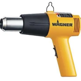
Figure 4.2: Heat Gun [42]

The heat gun analyzed was a basic consumer model in the 1200 W power range with two heat settings corresponding to 400 °C and 540 °C (Tout), based on the assumption of a 20 °C

operating environment (Tambient). The current draw of the device in operation was measured,

25 specific heat of air at constant pressure (cp) of 1.0 J/(g-K) was assumed for all calculations in

this section.

Step 1: Collect Stakeholder Specifications

For component-level excesses to be meaningful and useful in the design process, they must be relatable to specifications as defined by system stakeholders. This is because the specifications are the quantified embodiment of stakeholder needs, and are what is expected to change in response to future needs. Numbers chosen to complete the specifications should be target values (the minimum that any design is expected to yield). These are available to designers in the embodiment design phase. The product of this step is a requirements list of quantified specifications in engineering language. These comprise the datums against which system level excesses are measured.

Case study example

In the absence of direct customer needs information, it was assumed that the customer needs were captured by the company producing the heat gun. Therefore, a subset of the customer needs are:

• Produce air sufficiently hot to melt plastic, desolder circuits, loosen floor tile adhesive, etc.

• Produce enough heated air flow to quickly accomplish tasks • Be lightweight enough to use with one hand

• Be compatible with North American household electrical circuits

Based on the above customer needs, the following specifications were determined: • Maximum output temperature ≥ 540 °C

• Total mass ≤ 500 g • Power ≥ 1.0 kW • Power ≤ 1.4 kW

26 minimum bound for power is 1000 W. Assuming a mass flow rate of 2 g/s of air (the same as the example heat gun consumes) a 1000 W input results in an output temperature of 743 K or 520 °C as given in Equations 4.1 and 4.2.

𝑇_𝑜𝑢𝑡 = 𝑇_{𝑎𝑚𝑏𝑖𝑒𝑛𝑡}+ 𝐼 ∙ 𝑉

𝑐_𝑝∙ 𝑚̇ ( 4.1 )

= 293 K + 1000

J s

1.0_{𝑔𝐾 ∙ 2}𝐽 𝑔_𝑠 = 793 𝐾 = 520 °𝐶 ( 4.2 )

In this equation, Tout is the output temperature of the heat gun, Tambient is the ambient air

temperature, I is the current feeding the heating coils, V is the main voltage, cp is the specific

heat of air at constant pressure, and 𝑚̇ is the mass flow rate of air.

The upper bound was established based on the assumption that the user will be powering it from a household circuit with a 15A breaker, that the breaker’s maximum continuous load is 80% of its rating per code [43], and that nothing else is operating on the circuit while the heat gun is being used. Since the vast majority of the current drawn by the heat gun is a resistive load, the assumption was made that

𝑃𝑚𝑎𝑥 = 15 𝐴 ∙ 120 𝑉 ∙ 80% = 1440𝑊 ( 4.3 )

Step 2: Identify System Architecture and Relationships

The first decision made by the designer is the overall level of abstraction desired in the system excess map, or in other words, the intended level of assembly to be mapped. This decision is informed partly by the requirements list, which may pertain more to some components/subsystems than others. A starting point is the highest level of abstraction that separates the major components displaying modular behavior.

27 abstraction of their representation [44]. Different subsystems may be described at different levels of abstraction for these reasons. Figure 4.3 demonstrates how a component representation can be expanded (or condensed) when needed in the course of mapping excess.

Subsystem Compatibility

Flow

Functional Flow

Component A

Component B

Component C

Functional Flow Compatibility

Flow

More Detail

Less Detail

Figure 4.3: Variable Level of Abstraction

28

Type Excess [Units] (Total Capacity)

Type Type

Type

Type Excess [Units] (Total Capacity)

Type

Component

Functional Flows

Inbound Compatibility

Flows

Primary Block

Outbound Functional

Flows

Figure 4.4: Excess Map Segment for General Architecture

First, each component is considered individually and the types of compatibility (input) and functional (output) flows are determined. This is done by consulting the original design information for the purposes and requirements of each component. Then, the values associated with these flows are quantified.

Some compatibility flows, such as an input of electrical energy that is converted by a component to an output of heat energy, are a function of the required functional flow values and will change if the functional requirements of the component are later altered. Other compatibility flows that are static properties of components (typically Storage class excesses such as loads or geometric requirements) are updated only if a different component is selected as replacement. Some components will produce excesses that are linked; i.e. utilizing one of the associated excesses will diminish another. This is indicated by drawing a double-ended arrow between the two excess blocks.

29 component in turn and consider every possible excess from the Excess Basis. This forces the designer to consider the task of identifying relationships from a different perspective, and allows those that were not immediately clear to be captured. This activity reveals relationships driven by inter-component requirements that may have remained implicit, such as the requirement of a container to withstand the heat generated by internal components.

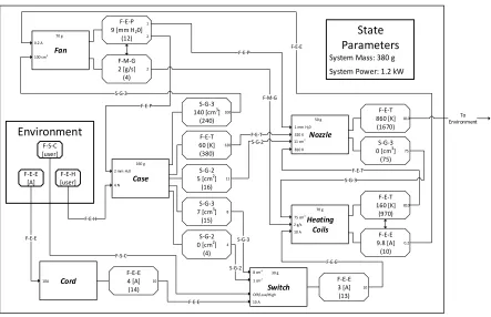
Case study example

The physical boundaries of the heat gun were used to define the control volume. Specifically, any energy or signal passing into or out of the device, whether electrical energy from the power grid, human energy from the operator, or heat from the nozzle, was viewed as crossing the control volume. The components selected were the self-contained subsystems: namely the case, controller, cord, fan, heating coils, and nozzle.

An important activity of this step is the selection of appropriate units for excess. The excess basis intentionally does not assign units to excess types, since the most appropriate/useful way to express a particular excess type is dependent on the situation at hand. In the case of a heat gun, it would be valid to describe the thermal excess of the nozzle in terms of Watts of dissipated energy. Most meaningful, however, is expressing the energy of the heated air in terms of its temperature in degrees Kelvin. This avoids the intermediate calculations that would be required to relate the thermal energy to a temperature threshold for the constituent materials of the heat gun.

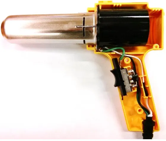
30 Figure 4.5: Disassembled Heat Gun

Case

31 The case, shown in Figure 4.6, is made of plastic and disassembles to three pieces: two mirrored grip/receiver pieces and a collar that locks onto the assembled grip. Assuming it is made of ABS plastic, the maximum use temperature is 105 °C [45]. The grip section provides volume for the switch to occupy and surface area for the switch to protrude through so that the user can interact with it. The barrel section provides volume to the fan and nozzle and withstands heat from the nozzle. Therefore, two distinct excess blocks for volume (Storage, Geometric, Volume or S-G-3 per the abbreviations listed in Table 3.1) and two distinct excess blocks for area (S-G-2) are shown since the spaces being occupied by the components are in separate locations in the case.

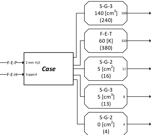
Finally, a thermal energy excess block (Flow, Energy, Thermal or F-E-T) is shown due to the dependence of the nozzle on the ability of the case to hold it at operating temperature. This highlights an important aspect of the excess relationships: their directionality is based on functional dependence, but this does not necessarily correspond to the direction of the involved physical flows. The actual heat is flowing from the nozzle to the case, but the nozzle is dependent on the ability of the case to withstand its steady-state operating temperature. Therefore, the relationship is shown as a functional flow of the case (its ability to withstand heat) satisfying a compatibility flow of the nozzle. The component and excess blocks for the case are shown in Figure 4.7.

32 F-E-H

F-E-P

Case

S-G-3 140 [cm3]

(240) 100

F-E-T 60 [K]

(380) 320

S-G-2 0 [cm2]

(4) 4 S-G-3 5 [cm3]

(13) 8 2 mm H20

Support

S-G-2 5 [cm2]

(16) 11

Figure 4.7: Case Excess Map Contribution

Cord

The cord and internal wiring is three-wire (hot, neutral, and ground) 18 AWG and therefore capable of carrying up to 14 A of current [43]. It requires electrical energy (F-E-E) from the environment and supplies electrical energy to the switch. The component and excess blocks for the cord are shown in Figure 4.8. The current passed on to the switch is 10 A, meaning that 4 A of excess current remains.

F-E-E 4 [A] (14)

10 Cord

10A

F-E-E

33 Switch

Figure 4.9: Heat Gun Switch

The switch, shown in Figure 4.9, is a three position sliding switch with positions corresponding to sequential markings of Off, Low, and High. In the Off position, the circuit is open. In the Low position, the circuit is fed by the current of the hot wire passed through a diode, making the current half-wave rectified. Therefore, the root-mean-squared (RMS) voltage fed to the heating coils and fan drops significantly; additionally, the diode itself drops the voltage by 0.6-0.7V [46] but this is insignificant compared to the adjusted half-wave rectified VRMS of

𝑉_𝑅𝑀𝑆 =𝑉𝑝𝑒𝑎𝑘

2 =

170 𝑉

2 = 85 𝑉 ( 4.4 )

(F-E-34 E). The component and excess blocks for the switch are shown in Figure 4.10; their values are based on the switch’s function in the High position.

S-G-3

F-E-E S-G-2 F-S-C

F-E-E 3 [A] (13)

10 Switch

8 cm3

10 A 4 cm2

Off/Low/High

Figure 4.10: Switch Excess Map Contribution

Heating Coils

Figure 4.11: Heat Gun Heating Coils

35 the excess of electrical flow that could be fed to the fan is correlated with the maximum air temperature that the coils can yield.

The airflow values are calculated as shown in Equation 4.5. Based on these numbers, the mass air flow through the heat gun at maximum temperature is approximately 2 g/s.

𝑚̇ = 𝑃

𝑐_𝑝∙ (𝑇_𝑜𝑢𝑡− 𝑇_{𝑎𝑚𝑏𝑖𝑒𝑛𝑡}) ( 4.5 )

The heating coils require 75 cm3 of volume (S-G-3) from the nozzle, 2 g/s of airflow (F-M-G) from the fan, and 10 A of electrical energy (F-E-E) from the switch. The component and excess blocks for the heating coils are shown in Figure 4.12. They supply 810 K of thermal energy (F-E-T) out of a maximum 970 K to the nozzle and 0.2 A of electrical energy (F-E-E) out of a maximum 10 A to the fan.

F-E-E S-G-3 F-M-G

F-E-T 160 [K]

(970) 810

Heating Coils

75 cm3

2 g/s 10 A

F-E-E 9.8 [A]

(10) 0.2

36 Fan

Figure 4.13: Heat Gun Fan

The fan, shown in Figure 4.13, is a 12V axial flow fan that delivers air from the case inlets to the heating coils. The fan has an integrated rectifier, which allows the AC current received from the coils to be converted to DC current. The fan, at its operating RPM, supplies approximately 2 g/s of airflow (F-M-G) to the heating coils and overcomes an estimated 3 mm H20 of static pressure (a relationship of F-E-P) imposed by the case and nozzle. The values of

estimated static pressure imposed by the case and nozzle were obtained by referencing the static pressure that commercially available 12V fans are capable of overcoming and examining the relative flow restrictions imposed by the case and nozzle. It is assumed that the rotational speed of the fan motor can be as much as doubled by adjusting the voltage fed to the fan, thereby creating excess in the two relationships. The fan affinity laws [50] for a constant diameter fan, shown in Equations 4.6–4.7, demonstrate how these excesses are linked, i.e. increasing airflow reduces the amount of additional static pressure that the motor can overcome. Volume flow rate is denoted by q and pressure by p. This linkage is indicated by a double-sided arrow between the excess blocks shown in Figure 4.14.

𝑞₁

𝑞₂ =

𝑅𝑃𝑀₁

37

𝑝₁

𝑝₂ = (

𝑅𝑃𝑀₁

𝑅𝑃𝑀₂)

2

( 4.7 )

The fan requires 0.2 A of electrical energy (F-E-E) from the heating coils and 100 cm3 of volume (S-G-3) from the case. It supplies 1 mm H2O of pressure (F-E-P) to the nozzle and 2

mm H2O to the case out of a maximum of 12 mm H2O pressure. It supplies 2 g/s of airflow

(F-M-G) to the heating coils out of a maximum of 4 g/s. These two excesses are linked, meaning that if one is utilized the available excess in the other will decrease. Therefore, a double sided arrow is shown between the two excess blocks.

Fan

F-E-P

9 [mm H20]

(12)

1

F-M-G 2 [g/s]

(4)

2 2 0.2 A

100 cm3

F-E-E

S-G-3

Figure 4.14: Fan Excess Map Contribution

Nozzle

Figure 4.15: Heat Gun Nozzle

38 restriction on the airflow (F-E-P); however, its exit geometry is very similar to that of the heating coils, so the impact is minimal. The static pressure imposed by the nozzle is assumed to be 1 mm H2O. The nozzle also requires cross sectional area (S-G-3) from the case, the ability

for the case to withstand a temperature of 30 °C above the ambient due to heat flow from the nozzle (F-E-T), and heated airflow (F-E-T) from the heating coils. The component and excess blocks for the nozzle are shown in Figure 4.16.

The nozzle requires 1 mm H20 of pressure (F-E-P) from the fan, 320 K of thermal energy

(F-E-T) from the case, 11 cm2 _{of area (S-G-2) from the case, and 810 K of thermal energy}

(F-E-T) from the heating coils. It supplies 810 K of thermal energy to the environment out of a maximum of 1670 K, and 75 cm3 of volume (S-G-3) to the heating coils (the maximum available).

F-E-T F-E-T F-E-P

F-E-T 860 [K]

(1670) 810

Nozzle

1 mm H20

320 K

810 K

S-G-3 0 [cm3]

(75) 75 11 cm2

S-G-2

Figure 4.16: Nozzle Excess Map Contribution

Step 3: Assemble Excess Map

39 components are not shown on the map; they may be encoded in a computational environment such as Simulink [52] or manually calculated.

Case study example

The process of assembling the excess map requires ensuring that the functional flows are matched with the correct compatibility flows. Components are presented with their summarized functional and compatibility flows in Table 4.1.

Table 4.1: Heat Gun Component Excesses

Component Compatibility Flows Functional Flows

Case Flow-Material-Gas Flow-Energy-Human

Flow-Energy-Thermal Storage-Geometric-Volume (2)

Storage-Geometric-Area (2)

Switch

Flow-Signal-Control Flow-Energy-Electrical Storage-Geometric-Volume

Storage-Geometric-Area

Flow-Energy-Electrical

Cord Flow-Energy-Electrical Flow-Energy-Electrical

Fan Storage-Geometric-Volume Flow-Energy-Electrical

Flow-Material-Gas Flow-Energy-Pneumatic

Heating Coils

Flow-Material-Gas Storage-Geometric-Volume

Flow-Energy-Electrical

Flow-Energy-Thermal Flow-Energy-Electrical

Nozzle

Flow-Energy-Thermal (2) Storage-Geometric-Area Flow-Energy-Pneumatic

Flow-Energy-Thermal Storage-Geometric-Volume

40 Step 4: Identify State Parameters

Some of the datums created from system specifications will be relatable to single component outputs, such as ‘10 MW of electrical power’ would be for a single-generator system. However, the satisfaction of other specifications will be functions of multiple components, as in the case of ‘total mass must be less than 5 kg’. To verify satisfaction, state parameters (equations that are functions of multiple components’ characteristics) are defined. These parameters are indicated in a block labeled ‘State Parameters’. Information is drawn from component blocks and flows, but arrows are not required so that visual complexity of the map is not increased. Component properties that do not interact with excess flows but are relevant to state parameters are denoted within their respective block.

Case study example

41 Environment F-E-E [A] F-E-H [user] F-S-C [user] F-E-T 160 [K] (970) 810 Heating Coils

75 cm3

2 g/s

10 A _F-E-E

9.8 [A] (10) 0.2 F-E-E 4 [A] (14) 10 Cord 10A Fan F-E-P 9 [mm H20]

(12) 1 F-M-G 2 [g/s] (4) 2 2 0.2 A

100 cm3

F-E-E F-M-G S-G-3 S-G-3 Case S-G-3 140 [cm3_]

(240) 100 F-E-T 60 [K] (380) 320 S-G-2 0 [cm2_]

(4)

4

S-G-3 7 [cm3]

(15)

8 2 mm H20

4 N

F-E-P

S-G-2 5 [cm2]

(16) 11 F-E-H F-E-E F-S-C F-E-E S-G-3 S-G-2 F-E-E 3 [A] (13) 10 Switch

8 cm3

10 A

1 cm2

Off/Low/High F-E-E S-G-2 F-E-T 860 [K] (1670) 810 Nozzle

1 mm H20 320 K 810 K F-E-T F-E-T F-E-P S-G-3 0 [cm3_]

(75)

75

11 cm2

To Environment 160 g 30 g 70 g 70 g 50 g State Parameters

System Mass: 380 g

System Power: 1.2 kW

Figure 4.17: Heat Gun Excess Map

Evaluating System Level Excess

For a system excess map that incorporates equations relating component outputs and inputs, it is possible to query the map and determine the extent that system specifications may be exceeded; these values will be the system excesses. Additionally, for each top-level excess, it is possible to determine which component is at an excess threshold and may limit performance changes.

Case study example

Excess (X) in a specification is evaluated using the relationship in Equation 4.8.

42 For the system in question, it was found that there exists 120 g excess in terms of allowable mass, using Equation 4.8 along with Equation 4.9. For excesses driven by state parameters, the ‘available’ amount is considered to be the bound on the state parameter, in this case 500 g.

𝑚𝑡𝑜𝑡𝑎𝑙 = 𝑚𝑐𝑎𝑠𝑒 + 𝑚𝑓𝑎𝑛+ 𝑚𝑐𝑜𝑖𝑙𝑠+ 𝑚𝑛𝑜𝑧𝑧𝑙𝑒 ( 4.9 ) The maximum possible output temperature is 700 °C (an increase of 160K over the current high output temperature), which is limited by the heating coil assembly. The switch, rated at 13 A, is the lowest-amperage component that feeds electrical energy into the system; therefore, the electrical components also limit the heat gun to a maximum temperature of approximately 700 °C as detailed in Equations 4.10 and 4.11 below. Note that 12.8 A is used as the maximum current value because roughly 0.2 A is consumed by the fan, thereby reducing the total current that can be expended in the heating coils slightly.

𝑋 = 12.8

𝐴

𝑠 ∙ 120𝑉 1.0_{𝑔𝐾 ∙ 2.3}𝐽 𝑔_𝑠 −

9.8𝐴_{𝑠 ∙ 120𝑉}

1.0_{𝑔𝐾 ∙ 2.3}𝐽 𝑔_𝑠 ( 4.10 )

=1540

𝐽 𝑠 2.3_𝐾𝑠𝐽 −

1180_𝑠𝐽

2.3_𝐾𝑠𝐽 = 160 K ( 4.11 )

Though a higher temperature could also be achieved at the same amperage by lowering the mass flow rate, an end user might not perceive any performance improvement if the total power remained constant. Regarding the power specifications, the system might consume 200 W more or less and still meet both. The power value for the system was determined from Equation 4.12, where I is the current passing through the switch.

𝑃 = 𝐼𝑉 ( 4.12 )

43 Map Quality and Criteria for Update

Two conditions can arise that require the excess map to be updated. Either the architecture changes in a way that alters the presence and/or arrangement of components depicted in the map, or system specifications have been added or removed. The addition or removal of specifications could alter the map by affecting the components and/or relationships that must be represented. However, an already present specification that is modified could change the amount of excess indicated by the map, but will not require the map to be altered. Rather, a modified need results in re-querying the map to determine how excesses are affected. The following sections implement and demonstrate the steps of the excess mapping process.

Case Study 1 Conclusion: Heat Gun Evolution Examples

Two examples of potential evolutions for the heat gun are given here to demonstrate the information made available to the designers by the excess map.

Heat Gun Evolution 1: Replace Tri-Mode Switch with Variable Voltage Switch

A possible future need for the heat gun is for the heat output to be made continuously variable. This could be accomplished by replacing the original switch, capable only of operating the heat gun in ‘low’ and ‘high’ temperature modes, with a dial switch that can vary the voltage across the entire possible range (with the minimum voltage set so that the 12 V nominal fan motor does not stall and thereby allow the heating coils to overheat and damage the device).

The feasibility of such a modification can be investigated by consulting the Switch block of Figure 4.17 and ensuring that a candidate replacement switch satisfies all existing functional flow requirements and can operate within the compatibility flow limits imposed by the supplying components to prevent change propagation. This means that a replacement switch must be able to pass at least 10 A (the present design amperage), must fit within 13 cm3 _inside

the case, and must occupy less than 4 cm2 _{of area on the case surface for the user to interface.}

44 for everything from a simple component exchange such as this to a more complicated alteration that can affect multiple components, as discussed in the next evolution.

Heat Gun Evolution 2: Increase Output Temperature to 750 °C

Another potential future need for the system is for the output temperature to be increased from 540 °C to 750 °C (1020 K) meaning a ΔT of 730 K. Consulting the system excess map of Figure 4.17, it is apparent that the nozzle can tolerate the evolution. Additionally, assuming that the ΔT between the case temperature and ambient air is linearly correlated with the ΔT imparted to the airflow, the new case temperature will be 62°C, as shown in Equation 4.13. This is still well within the maximum temperature of 105°C.

ΔT_case

ΔT_airflow= const = 30 K

520 K=

𝟒𝟐 𝐊 730 K

( 4.13 )

However, the heating coils must be modified as their current maximum operating temperature is 700 °C. Also, assuming that the airflow rate is to remain constant, the flows of electrical energy must be considered. A ΔT of 730 K requires an energy input of 14 A. Therefore, the switch (rated at 13 A) must be upgraded, but there is sufficient excess in the cord.

I =𝑚̇ ∙ 𝑐𝑝∙ Δ𝑇

𝑉 =

2.3𝑔_{𝑠 ∙ 1.0𝑔𝐾 ∙ 730𝐾}𝐽

120𝑉 = 12 𝐴

( 4.14 )

Upgrades to the switch and heating coils are governed by the available compatibility flows (volume and area for the switch, and volume for the heating coils) if changes are not to propagate to additional components in the design.

Case Study 2: Coffee Maker

45 Figure 4.18: Coffee Maker [53]

This particular model was an automatic drip brewer producing up to twelve 5 fl. oz. cups of coffee using a basket filter. It was operated using an on-off switch without automatic shutoff functionality. The carafe was heated from below, maintaining the coffee at brewing temperature indefinitely.

Coffee Maker Excess Map Creation

Step 1: Collect Stakeholder Specifications

The coffee maker satisfied the following customer needs: • Brew coffee

• Keep coffee hot after brewing • Brew enough coffee for a family • Brew coffee quickly

• Be safe to use and operate

46 The corresponding specifications are:

• Deliver water at ≥ 93°C to coffee

• Maintain coffee at brewing temperature (93°C) • Brew at rate of ≥ 150 mL/min

• Brew up to 1.8 L of coffee

• Limit heating element temperature to ≤ 240 °C in emergency • Power ≤ 1.4 kW

The brewing rate specification translates to brewing an entire pot (1.8L, or twelve 5 fl. oz. coffee cups) of coffee within 12 minutes. The power specification was set as in Equation 4.3.

Step 2: Identify Architecture, Appropriate Subassemblies, and Relationships

The system boundaries were determined based on the operation of the system between when it is turned on and off. Therefore, it was assumed that water is already in the reservoir when the system is turned on and that the system remains on until the last cup of coffee is poured from the carafe. The components that display modular behavior are the body, cord, brew basket, heating element, hot plate, and carafe. Pertinent to the following discussion is the specific heat of water at constant pressure, cp = 4.19 J/(g-K), and the assumption that the tap

47 Body

Figure 4.19: Coffee Maker Body

48 temperature is 135°C [54]. The component and excess blocks for the body are shown in Figure 4.20.

Body

S-G-2 0 [cm2]

(110)

110

S-G-3 0 [L] (1.9)

1.9

S-G-3 0 [cm3]

(860)

860

F-M-L 12.4 [mL/sec]

(15)

2.6 363

F-E-T 45 [K]

(408) S-M-L 0.2 [L]

(2.0)

1.8

S-G-2 0 [cm2]

(2)

2

Figure 4.20: Body Excess Map Contribution

Cord