Introduction to the bootstrap world

(1)

Introduction to the Bootstrap World

Dennis D. Boos

Statistical Science, Vol. 18, No. 2, Silver Anniversary of the Bootstrap. (May, 2003), pp. 168-174.

Stable URL:

http://links.jstor.org/sici?sici=0883-4237%28200305%2918%3A2%3C168%3AITTBW%3E2.0.CO%3B2-8

Statistical Science is currently published by Institute of Mathematical Statistics.

Your use of the JSTOR archive indicates your acceptance of JSTOR's Terms and Conditions of Use, available at

http://www.jstor.org/about/terms.html. JSTOR's Terms and Conditions of Use provides, in part, that unless you have obtained prior permission, you may not download an entire issue of a journal or multiple copies of articles, and you may use content in the JSTOR archive only for your personal, non-commercial use.

Please contact the publisher regarding any further use of this work. Publisher contact information may be obtained at

http://www.jstor.org/journals/ims.html.

Each copy of any part of a JSTOR transmission must contain the same copyright notice that appears on the screen or printed page of such transmission.

The JSTOR Archive is a trusted digital repository providing for long-term preservation and access to leading academic journals and scholarly literature from around the world. The Archive is supported by libraries, scholarly societies, publishers, and foundations. It is an initiative of JSTOR, a not-for-profit organization with a mission to help the scholarly community take advantage of advances in technology. For more information regarding JSTOR, please contact [email protected].

(2)

O Inst~tuteof Mathematical Statist~cs. 2003

Introduction to the Bootstrap World

Dennis D. Boos

Abstract. The bootstrap has made a fundamental impact on how we carry out statistical inference in problems without analytic solutions. This fact is illustrated with examples and comments that emphasize the parametric bootstrap and hypothesis testing.

Key words and phrases: Statistical inference, hypothesis testing, confidence intervals, resampling, resamples.

1. INTRODUCTION

What is the bootstrap? It is a general technique for estimating unknown quantities associated with statistical models. Often the bootstrap is used to find

( I ) standard errors for estimators,

(2) confidence intervals for unknown parameters or (3) p values for test statistics under a null hypothesis.

Thus the bootstrap is typically used to estimate quantities associated with the sampling distribution of estimators and test statistics.

Recall that a statistical model is essentially a set of probability distributions that attempts to describe the true state of nature and the related random data available to understand that true state. The goal of statistical inference is to choose one of these probability distributions and give some notion of the uncertainty of that choice [usually by means of (I), (2) or (3) above]. In other words, we make inferences about unknown popu- lations (represented by statistical models) from sample data. The bootstrap, first introduced by Efron in 1977, is an important tool in making such inferences, espe- cially in complicated models.

So, we have a set of distributions

5'

and one dis- tinguished member Po that describes the true state of nature and the available data. Any of the above items (1)-(3) could be described as functionals Q ( P o ) , and the bootstrap estimate is Q(P^), where

P^

is an es- timate of Po. If

5'

is indexed by a finite-dimensional parameter 6 , then the model is called parametric and use of Q ( P ) is called a parametric bootstrap. Oth-

Dennis D. Boos is Professor of Statistics, North Carolina State University, Raleigh, North Carolina 27695-8203(e-mail: boos @stat.ncsu.edu).

erwise the term nonparametric bootstrap is typically used (even for semiparametric models like regression models with unknown error distribution).

This "plug-in" description is deceptively simple. The functional approach to estimating parameters like the

-mean T ( F ) =[ x d F ( x ) by T(Fn)

= X =

J x d F n ( x ) , where Fnis the empirical distribution function, was al- ready well known by 1977. In fact, an elegant asymptotic theory for T ( F , ) was available (see Serfling, 1980, Chapters 6-8). However, when Efron introduced the bootstrap in 1977, it was a truly novel idea even if in hindsight we can describe it simply as a functional. The key theoretical difference is that the bootstrap functionals are much broader and more complicated than functional~ like T ( F ) =[x d F(x). In fact, the most basic bootstrap functional is a sampling distribution itself.

I think the real reason the bootstrap was so path- breaking and has remained so popular is that Efron described it mainly in terms of creating a "bootstrap world," where the data analyst knows everything. That is, in this parallel world the true sampling design of the data is reproduced as closely as possible and unknown aspects of the statistical model are replaced by sample estimates. In this world, the data analyst can obtain any quantity of interest by simulation. For example, if the variance of a complicated parameter estimate in this world is desired, just computer generate

(3)

169

INTRODUCTION TO THE BOOTSTRAP WORLD

estimate. Thus we create a bootstrap world where any- 2. EXAMPLES

thing can be computed, at least up to Monte Carlo error. Those true quantities calculated in the bootstrap world are estimates of the parallel quantities in the real world. In effect this bootstrap world simulation approach opened up complicated statistical methods to anybody with a computer and a random number generator. Ran- dom variable calculus can be replaced by computing power. (I can hear groans about all the possible mis- uses. The same can be said about standard statistical software packages, but few people would doubt their importance.)

How important is the bootstrap resampling technique in statistical inference? First we need to separate the practical, everyday world from the research world that results in journal articles. In the everyday world, noth- ing can compare to the impact of statistical packages like SAS and SPSS, but as far as I can tell, SAS has only one PROC that directly uses the bootstrap (PROC MULTTEST). Splus has a general bootstrap program, but it is not automatic. Moreover, I contend that a ma- jority of practical statistical problems are handled by analysis of variance or regression for which standard methods are usually adequate. Thus, in terms of overall usage, the percentage of analyses that use bootstrap resampling is fairly low. On the other hand, I will try to show in the examples below, that in almost any problem that is slightly nonstandard, it could be helpful to use the bootstrap. When packages that have the bootstrap are as easy to use as StatXact, then we will see a huge rise in practical usage.

In the world of journal articles, the bootstrap has had a tremendous impact. Typing "bootstrap" into the IS1 Web of Science topic search resulted in 6,248 articles (and growing every day-a few weeks earlier it was 6,212). More than half of the 2000 and 2001 articles that cited Efron (1979) were from nonstatistical journals. So the bootstrap is making a large impact outside the statistics mainstream as well. Personally, I think the use of the parametric bootstrap in all kinds of analyses is going to grow in the future. In fact, I see some analogies between the parametric bootstrap in frequentist inference and Markov chain Monte Carlo methods in Bayesian analysis.

The rest of this article consists of two sections. The first section is a series of examples that I hope illus- trates the ubiquity of the bootstrap; the first and second examples came directly from my own consulting. Then the final section discusses a number of issues that arise in using the bootstrap in the context of hypothesis testing.

EXAMPLE1. A masters student in civil engi- neering wanted to model the relationship between watershed area and the maximum flow over a 100 year period at gauging stations on rivers in North Carolina. He had a model R =k ~ v - l that related the 100 year maximum flow rate at a station (R) to the watershed area ( A ) at the station; k and rj are unknown parame- ters. Taking logarithms leads to a simple linear model. He had values of A for 140 stations, but the R measure- ment for each station was the maximum flow during the time the station had been keeping records. These lengths of time varied between 6 and 83 years, so they really were not comparable and also were not appropriate for the maximum over 100 years.

I discovered that the student could get yearly maximums for a number of stations. The data in Table 1 are n = 35 yearly maximum flow rates at one particular station. Assuming year-to-year independence for the yearly maximums, the distribution function of the maximum of 100 yearly maximums is P(R(loo) F

t) = [F(t)]loO, where F(t) is the distribution function of a single yearly maximum. I proposed that we estimate the median, say to, of the distribution function [F(t)]loO to be used as the response variable in the regression model. Setting [F(to)]loo = 112 implies that F(to) = (1/2)0.01 =0.993. Thus, to is actually the 0.993 quantile of the yearly maximum distribution. Be- cause the sample sizes were too small to estimate this quantile nonparametrically, I suggested that we assume a parametric model for the yearly maximum. So, for the data of Table 1, I assumed a location-scale extreme value model that had distribution function

I confirmed this assumption with a quantilequantile (QQ) plot and then fit the data by maximum likelihood, obtaining

j2

=4395.1 and B = 1882.5. The estimate of the 0.993 quantile is then

TABLE1

(4)

Using the inverse of the estimated Fisher information and the delta method applied to the above function, I obtained a standard error of 1375.3. The idea would be for the student to do this estimation at a number of stations and possibly use the standard errors as weights in the regression fit.

The classical tools used here are quite adequate: QQ plot, maximum likelihood and delta method. How- ever, let us see what the bootstrap can do. I first confirmed the extreme value assumption by generating B = 100 data sets of size n = 35 from the fitted distribution and computed the Anderson-Darling (AD) goodness-of-fit statistic for each sample. Since 95 of these were larger than the value 0.178 for the data in Table 1 , the parametric bootstrap y value is 0.95. If the p value had been fairly small, I would have taken B to be much larger. The null distribution of AD for this situation has been tabled by Stephens (1977), but the bootstrap has made tabling such distributions obsolete. In fact, the bootstrap distribution here is exact up to Monte Carlo error, because the distribution of AD does not depend on the values of the parameter. This is true for any location-scale family. I also kept track of the bootstrap parameter estimates and the estimated 0.993 quantile for each bootstrap resam- ple. The mean of the quantile estimates was 13572.2, illustrating some negative bias of the estimate, since

13572.2 is smaller than 13729.2, the true value in the bootstrap world. The standard deviation of the quantile estimates was 1386.0, a parametric bootstrap standard error quite close to the parametric delta method value of 1375.3. Finally, I made a histogram and QQ plot of the 100 bootstrap 0.993 quantile estimates and ob- served that they are approximately normally distrib- uted (suggesting that the 0.993 quantile estimate from different stations will be a statistically well-behaved response variable in the linear regression). These bootstrap analyses are modest additions to the original analysis. but they do add some insight. For some folks, just avoiding the Fisher information and delta theorem calculus is attractive.

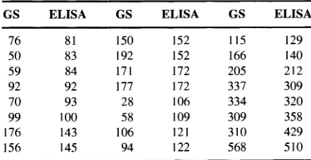
EXAMPLE2. A local Raleigh company came to me several years ago with data on two methods of detecting polychlorinated biphenyls (PCBs). They were developing a solid phase fluoroimmunoassay method that is called ELISA; the other method is refered to as GS for gold standard, because its results were accepted as truth. Figure 1 displays the data, the

FIG. 1. Two methods for detecting PCBs overlaid with the least squares line.

n =24 pairs of (GS, ELISA) values given in Table 2. The company was interested in detecting PCB levels of 200 ppb (parts per billion) or more using an "action limit" of 100 ppb for their ELISA method. That is, they planned to declare that PCBs were present whenever ELISA was greater than or equal to 100.

After some discussion, we determined that the company wanted the probability of a false negative when GS = 200, P (ELISA < 1001 GS =200). In screening test terminology, this probability would be 1 minus the

sensitivity of the test. They also were interested in the

probability of a false positive (1 minus the speczjicity

of the test) for different levels of GS. Since all of these calculations are similar, I will focus here on the sensitivity.

To make the problem simple, I decided to model the ELISA results as a linear function of GS with normal homogeneous errors,

(1) ELISA = a

+

B(GS)

+

aZ,

where Z is a standard normal random variable.

T A B L E2

GS and ELISA valuesfor 24 samples

(5)

171

Then

P(ELISA < 1001 GS =200)

= P ( a +/3(GS) + o Z < lOOIGS= 200) 100 -a -

/3

(200)

(2) = P ( Z <

a

)

loo -a -B(200)

=

@(

a

1.

where @ is the standard normal distribution function. Since (a,/3, a ) were unknown, I used the least squares estimates from a fit to the data in Figure 1 to substitute in (2). The estimate of (2) was 0.002, but how should the variation due to the parameter estimates be taken into account? One could use the joint asymptotic normal distribution of the least squares estimates and the delta method to get a standard error for the estimate and an approximate confidence interval, but it was much simpler to just generate 10,000 samples from the model (1) with the least squares estimates in place of (a,

/3,

a ) . This is a parametric bootstrap. The bootstrap standard error was 0.005 and the upper 95% probability bound was 0.013 using the percentile method. I worried a bit about the normality assump- tion, and decided to try a t distribution with 5 degrees of freedom as an alternative to the normal distribution. The probability estimate was then 0.007 with bootstrap standard error 0.009 and upper 95% probability bound of 0.023. So there is clearly some sensitivity to the normal assumption. (Actually, it appears that a Weibull distribution might be more appropriate for the errors, but I did not pursue distributional alternatives further because of time and money.) One could also worry about variance heterogeneity and other model inade- quacies or use a better bootstrap confidence interval method.

The key point I want to make is how easy it was to carry out the bootstrap analysis (in Splus, actually) in comparison to the classical delta method. Moreover, I was able to check on sensitivity to the normality assumption with a very slight change in my program.

EXAMPLE3. Chen, Kodell and Gaylor (1996) dis- cussed risk assessment for increasing doses of toxic agents based on continuous responses. Their second example is a study that relates glucose levels in mice who were fed various doses of carbonyl iron. The doses were 0, 15, 35, 50 and 100 dg/kg body weight of iron per day. Descriptive statistics reveal that the variance of the glucose response variable increases with

dose. (Actually, the authors ran a Bartlett test for homogeneity of variances. In my younger days I would have argued that they should have obtained a p value from the nonparametric bootstrap since Bartlett's test is so sensitive to the normality assumption; see Boos and Brownie, 1989. Here the heterogeneity is so strong that it does not matter.) Then, assuming normality for the responses and allowing each dose group to have its own standard deviation, they used maximum likelihood to fit a quadratic mean function of dose to al- low for a downturn at high doses. They then gave a bias-corrected estimate (based on Taylor expansion) of "additional r i s k that is a function of the parameter estimates based on the normal distribution function. Finally, they gave three methods for obtaining confidence intervals for the quantity of interest, one of which is a nonparametric bootstrap. So, they have used the bootstrap once, but they also could have used it with Bartlett's statistic and for bias correction.

They also could have worried about the normality assumption (they did in a later article; see below), es- pecially since their procedures rely on it fairly strongly. My colleague Charles Quesenbeny gave exact procedures (Quesenberry, 1976) for testing normality in multiple samples, but I did not have the program at my fingertips. Instead, I just standardized each data value by subtracting its sample mean and dividing by its sample standard deviation. Then I pooled all 1 18 standardized values and computed the Anderson-Darling goodness-of-fit statistic. I obtained AD = 0.86. How- ever, what is the accompanying p value? I gener- ated B = 1000 sets of five samples and computed this AD statistic each time, resulting in a parametric bootstrap p value =0.022. This is not overwhelming evi- dence, but certainly there is some nonnormality. As in Example 1, the null distribution of AD does not depend on actual parameter values and thus the parametric bootstrap p value here is exact up to Monte Carlo error. Continuing the story, Razzaghi and Kodell (2000) also noticed the nonnormality in these data and proposed a mixture model. The distribution function of the jth observation in the i th dose group is

(6)

So, the main consideration is whether the overall model is adequate. To address this question I used the fitted model to generate parametric bootstrap samples and computed a new model adequacy statistic IOSA (in-and-out-of-sample) each time (see Presnell and Boos, 2002, for a description of the statistic). The

p value was 0.24 for B = 100, suggesting that the model is reasonable.

My conclusion from looking at these examples is that the bootstrap has potential uses in almost any problem. Whether it is used or not depends a lot on how easy it is to implement and whether there is an acceptable standard procedure available.

3. BOOTSTRAP SAMPLING FOR HYPOTHESIS TESTS

Since the bootstrap literature has not emphasized hypothesis testing very much, I thought it might be interesting to highlight some of the issues associated with resampling test statistics.

3.1 Correct Resampling for Hypothesis Tests

An understanding of bootstrap resampling for obtaining a standard error or confidence interval does not necessarily provide intuition concerning how to resam- ple in a hypothesis testing situation. The key point is that to get a p value, resampling must be performed under an appropriate null hypothesis, whereas for standard errors and confidence intervals, resampling is un- restricted.

To make this clear, consider the case of two independent samples X I , .

. .

,X, and Y1,.

. .

,Y,, and suppose that we are interested in the difference in population means, say

p x

-p y . For a nonparametric bootstrap confidence interval, we merely draw independent samples from the empirical c.d.f.'s or equivalently with replacement from the sets { X I ,

. . .

,

X,} and {Y1,.

. .

,Yn}, respectively. Instead, consider testing p~ -p y =0 with a t statistic, say the pooled

t statistic

t, =

(x-n/,i.;('+

rn

t),

where

2 (m -1)s;

+

(n -l > s y

S

P = m + n - 2 ,

2

Sx = -1 C ( X i -

m2.

m -1 j=1

2 I n

S y = -C ( y i -F12.

n - 1

1=1

The above method of resampling from each sample separately leads to a test with power approximately equal to the nominal level.

Why is that resampling method wrong? Resampling in the above fashion puts no restriction on the data and thus does not generate an approximation to the null distribution of the t, statistic. For confidence intervals for p x -p y , we do not want any restriction in the bootstrap world, but for the null distribution of t,, we need to force the means to be equal when drawing bootstrap samples.

One way to do this is to draw both samples with replacement from the pooled set { X I , .

. .

,X,, Y1,

. . .

,Y,}. By doing this, in the bootstrap world we have

created the null hypothesis

where P ( X * 5 t) is the distribution function of an X in the bootstrap world, P(Y* 5 t) is the distribution function of a Y in the bootstrap world and HN (t) is the empirical distribution function of the pooled set with N =m

+

n. In effect we are trying to test the real world hypothesis

where F and G are the distribution functions of the X and Y samples, respectively.

It might be worth pointing out that there is an exact permutation test available for (4), obtained by con- structing all N!/m!n! partitions of { X I , .

. .

,X,, Y1,

. . .

,Yn} into two samples of size m and n, respectively.

Then t, is computed for each partition; the empirical distribution of these N!/m!n! values is called the permutation distribution. The statistic t, for the original sample is then compared to this distribution to get exact tests and p values. This elegant approach was introduced by Fisher (1934); a firm theoretical foundation can be found in Hoeffding (1952).

(7)

173

distribution (see Hall, 1986b or 1992). For permutation tests, however, using different statistics often leads to the same result. For example, in the above problem, the permutation method applied to t p and to -

r

yields the same test.

To further illustrate these ideas, consider a larger null hypothesis than (4),

(5) H 0 : P x -PY = o ,

but with no other restrictions on the distributions except for finite second moments. This allows the distributions to have different variances and even totally different shapes. A suitable statistic might be Welch's t :

One way to create a bootstrap world with an appro- priate null hypothesis is to draw the X resamples with replacement from { X I-

X,

. .

.

,X , -

x}

and the Y re-samples from { Y 1-

Y ,

.

. .

,Y, -

Y}.

This forces the

X and Y distributions in the bootstrap world to have mean 0. Of course, we could add the same constant to both sets of resamples and not change the results (since

t , is invariant to such additions). It is easy to show that the bootstrap distribution of t, converges with proba- bility 1 to a standard normal distribution, the same lim- iting distribution as t, in the real world under the null distribution (5). Thus under ( 9 , the bootstrap p value converges with probability 1 to a uniform random variable. The permutation method cannot handle (5).

Other examples of creating null hypotheses in the bootstrap world can be found in Beran and Srivastava (1985), Boos, Janssen and Veraverbeke (1989) and Davison and Hinkley (1997, Chapter 4).

3.2 Definition of Bootstrap p Values and the "99 Rule"

Suppose that To is the value of a test statistic T computed for a particular sample. Then P (T

2

To

I

Ho) is the definition of the p value in situations where large values of T support the alternative hypothesis. If the null distribution of T is a discrete uniform distibution on some values t l ,

. . .

,tk (each value has probability Ilk), then the p value is just the proportion of ti's greater than or equal to To. In analogous fashion, when B resamples are made in the bootstrap world under an induced null hypothesis, define the bootstrap P value

{# of

Ti*

>

To}

PB = ,

B

where T;,

.

,T$ are the values of T computed from the resamples. This is the definition I prefer and is the one given by Efron and Tibshirani (1993, page 221). I should note, however, that Davison and Hinkley (1997, pages 148 and 161) and others prefer ( p B

+

I)/ (B

+

I).

Consider a situation where the statistic T is continuous and a parametric bootstrap will give the exact sampling distribution as B grows large (such as in Example 1). In this case, To, T;,

. . .

,T; are i.i.d., all (B

+

I)! orderings are equally likely and p~ has a discrete uniform distribution,

Thus, the test defined by the rejection region p~ 5 a has exact level a if (B

+

l ) a is an integer. For example, if a = 0.05, then P ( p B 5 0.05) = 5/(99

+

1) =

0.05 if B =99, but P ( p B 5 0.05) =6/(100

+

1) =

0.0594 if B = 100. So, for small B one should use values like B = 19,39 or 99 to get standard a levels. I call this the "99 rule" and note that simulation- based tests such as this are often called Monte Carlo tests (first suggested by Barnard, 1963). Hall (1986a) gave an approximate version of this result for the nonparametric bootstrap; thus the "99 rule" should be followed generally in bootstrap testing situations.

When analyzing a single data set, it is often possible to use a large B where there is very little difference between using B and B

+

1 (B = 1000 gives a rejection rate of 51/1001 = 0.051). However, for studying the power function of a bootstrap test, two Monte Carlo loops are required (the outer one for replicate samples of the true data situation; the inner one for the bootstrap procedure) and computations can be time consuming. Thus B =59,99 or 199 might be used to save time. Since the resulting power estimates are typically monotone increasing in B, one can adjust the estimates if B is taken to be small (see Boos and Zhang, 2000). Davison and Hinkley (1997, Section 4.5) use related arguments to justify the use of 99 resamples in the inner loop of a double bootstrap procedure to get adjusted bootstrap p values for a single data set.

3.3 Convergence of Parametric Bootstrap

P

Values

(8)

Recently, Robins, van der Vaart and Ventura (2000)

gave an interesting result for the parametric bootstrap. One conclusion for bootstrap p values from their The- orem 1 is as follows. If the test statistic T is asymptotically normal ( a ( 6 ) ,b2( 8 ) / n ) ,then under some fairly strong but general conditions, the parametric bootstrap p value is asymptotically uniform if a does not depend on I9 and asymptotically conservative otherwise. The context of the result is an article on p values for model adequacy, and the authors suggest that the conservative property is not appealing in that context. They may have a point, but I find the result comforting in terms of general usage of the bootstrap in hypothesis testing situations.

4. CLOSING REMARKS

The bootstrap is a fundamental statistical tool that can be used in almost any application. Clearly, it is most useful in complex situations where asymptotic approximations are difficult to compute or just not available. As computing power continues to increase, the routine use of bootstrap resampling will continue to grow.

ACKNOWLEDGMENT

I wish to thank Cave11 Brownie, longtime collabora- tor and friend, for helpful suggestions on this manu- script.

REFERENCES

B A R N A R D ,G. A. (1963). Discussion of "Spectral Analysis of Point Processes," by M. S. Bartlett. J. Roy. Statist. Soc. Ser: B

25 294.

BERAN,R. J . (1986). Simulated power functions. Ann. Statist. 14

151-173.

BERAN,R. J . (1988). Prepivoting test statistics: A bootstrap view of asymptotic refinements. J. Amer: Statist. Assoc. 83 687-697. BERAN,R. and SRIVASTAVA,M. S . (1985). Bootstrap tests and

confidence regions for functions of a covariance matrix. Ann.

Statist. 13 95-1 15.

Boos, D. D. and BROWNIE,C. (1989). Bootstrap methods for testing homogeneity of variances. Technometrics 31 69-82.

BOOS, D. D., JANSSEN,P. and VERAVERBEKE,N. (1989). Resampling from centered data in the two-sample problem.

J. Statist. Plann. Inference 21 327-345.

BOOS, D. D. and ZHANG,J . (2000). Monte Carlo evaluation of resampling-based hypothesis tests. J. Amer: Statist. Assoc. 95

486-492.

CHEN, J. J., KODELL, R. L. and GAYLOR, D. W. (1996). Risk assessment for non-quanta1 toxic effects. In Toxicology

and Risk Assessment: Principles, Methods, and Applications

(A. M. Fan and L. W. Chang, eds.) 503-513. Dekker, New York.

DAVISON,A. C . and HINKLEY,D. V. (1997). Bootstrap Methods

and Their Application. Cambridge Univ. Press.

EFRON,B. (1979). Bootstrap methods: Another look at the jackknife. Ann. Statist. 7 1-26.

EFRON,B . and TIBSHIRANI,R. J. (1993). An Introduction to the

Bootstrap. Chapman and Hall, New York.

FISHER,R. A. (1 934). Statistical Methods for Research Workers, 5th ed. Oliver and Boyd, Edinburgh.

HALL,P. (1986a). On the number of bootstrap simulations required to construct a confidence interval. Ann. Statist. 14 1453-1462.

HALL,P. (1986b). On the bootstrap and confidence intervals. Ann.

Statist. 14 1431-1452.

HALL, P. (1992). The Bootstrap and Edgeworth Expansion. Springer, New York.

HOEFFDING,W. (1952). The large-sample power of tests based on permutations of observations. Ann. Math. Statist. 23 169-192.

PRESNELL,B. and BOOS, D. B. (2002). The in-and-out-of- sample (10s) likelihood ratio test for model misspecification. Mimeo Series 2536, Institute of Statistics, North Carolina State University, Raleigh.

QUESENBERRY,C. P. (1976). On testing normality using several samples: An analysis of peanut aflatoxin data. Biornetrics 32

753-759.

RAZZAGHI,M. and KODELL,R. L. (2000). Risk assessment for quantitative responses using a mixture model. Biometrics 56

519-527.

R O B I N S , J., VAN DER VAART,A. and V E N T U R A ,V. (2000). Asymptotic distribution of p values in composite null models.

J. Amer: Statist. Assoc. 95 I 143-1 156.

SERFLING, R. J . (1980). Approximation Theorems of Mathemati-

cal Statistics. Wiley, New York.